Category: Biotechnology News

  • Highly multiplexed mammalian metabolic engineering with a shotgun approach

    Highly multiplexed mammalian metabolic engineering with a shotgun approach

    Main

    The ability to exert precise and predictable control over cellular behavior is a central goal of synthetic biology. In metabolic engineering, this control is often achieved by coordinating the activity of multiple transcription units (TUs), each consisting of a gene and its regulatory elements. Synthetic metabolic pathways are frequently constructed by transplanting coding sequences (CDSs) from diverse species into orthogonal hosts, thereby endowing them with new metabolic capabilities. This approach has yielded notable successes, including the development of cell-based alternatives to industrial manufacturing processes, the stabilization of pharmaceutical supply chains previously dependent on seasonal plant sources and the capture of atmospheric carbon dioxide to generate industrially valuable biomass1,2,3. While these strategies have been extensively demonstrated in microbial chassis, examples of metabolic engineering at this pathway scale in mammalian cells remain rare4,5, despite broad recognition that improved control of mammalian cell function could enhance cell therapies, produce increasingly complex biologics and improve the scalable manufacture of viral vectors6,7,8. Modern DNA synthesis technologies now make it possible to incorporate sequences from across the phylogenetic tree or de novo designed sequences, vastly expanding the functional landscape accessible to mammalian cells.

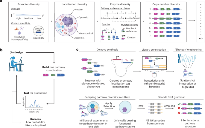
    Despite this promise, the limited examples of mammalian metabolic engineering can in part be attributed to the lack of foundational knowledge needed to guide metabolic pathway design. Given a target metabolic pathway and a target host cell type, one is faced with a series of complex design decisions, including the selection of CDSs, the configuration of regulatory elements, the intracellular localization of each encoded protein and the relative expression levels and stoichiometry of each TU required for optimal function (Fig. 1a). These variables create a vast combinatorial design space, yet there is little mechanistic understanding to guide optimal choices.

    Fig. 1: SGE expands DNA search space to sample many metabolic pathway solutions in parallel.

    a, Metabolic engineering benefits from increasing diversity across the different modules that make up TUs, including promoters, OLSs, enzymatic function, stoichiometry and copy number. b, Classical DBT frameworks in which pathways are tested in succession are inefficient in mammalian cells and other host chassis, which exhibit long doubling times or difficulties associated with engineering or delivering long DNAs that encode more complex biosynthetic pathways. c, SGE increases the scale of metabolic engineering by delivering barcoded individual TUs at high MOI such that each cell carries a unique pathway combination, thereby sampling much more pathway diversity. Following selection, cells displaying the desired phenotype can be sequenced to reveal TU combinations that conferred the desired function. Created in BioRender; Trolle, J. https://biorender.com/43izsew (2026).

    In fast-growing, genetically tractable microbial systems such as Escherichia coli (20-min doubling time) or Saccharomyces cerevisiae (90-min doubling time), the lack of mechanistic knowledge can often be mitigated through the design–build–test (DBT) framework, where metabolic pathways are rapidly constructed, tested and iteratively refined until satisfactory performance is achieved9,10 (Fig. 1b). Applying similarly complex metabolic engineering strategies in mammalian cells is far more challenging, primarily because of much longer doubling times (typically over 20 h), which drastically slows the pace of iteration.

    This limitation becomes increasingly severe as pathway complexity grows or as multiple functions are integrated into a single cell. While the final implementation of such complex functions may rely on recent advances in the synthesis and delivery of large DNA constructs to mammalian cells > 100 kb (ref. 11), these approaches are poorly suited for high-throughput screening, as delivering large DNA constructs into mammalian cells is highly inefficient. Modular combinatorial strategies, such as CLASSIC, offer a solution by enabling screening of ~105 constructs at the ~10-kb scale12 (2–3 TUs); however, there is a strong inverse relationship between DNA size and delivery success; it becomes exponentially more difficult to deliver larger constructs, rendering brute-force screening of complex synthetic designs impractical13.

    To overcome the limitations of experimental screening in mammalian systems, some metabolic engineering approaches incorporate computational screening of candidate interventions before testing in the lab12,14. Sophisticated transcriptomic databases and metabolic models have been developed for commonly used mammalian cell types, enabling the identification of epistatic metabolic functions and the design of complex multiple-knockout cell lines that improve bioprocessing and manufacturability of antibodies15,16,17. However, these models are typically trained on observational data shaped by natural evolution and are optimized for a narrow range of species and cell types commonly used in biomanufacturing. As a result, they are poorly suited for generative design, including scenarios involving the introduction of heterologous or entirely synthetic TUs. The design of TU arrays that comprise synthetic metabolic pathways adds yet another layer of complexity, beyond what these models can currently handle. Thus, synthetic data are needed—systematic, large-scale metabolic perturbations that can be used to train machine learning models capable of predictive and design-oriented applications18.

    Here, we introduce shotgun genetic engineering (SGE), a multiplexed approach to mammalian metabolic engineering that enables rapid discovery of complex pathway solutions and the creation of large-scale synthetic datasets for training predictive models. SGE leverages high-multiplicity integration of barcoded individual TUs from a pooled library, allowing distinct pathway variants to be randomly assembled within each cell. Because small DNA constructs are exponentially easier to synthesize, assemble and deliver, this design turns each cell into an independent experiment and enables millions of combinations to be screened in parallel. By selecting for cells with desired phenotypes and sequencing their associated barcodes, SGE bypasses the limitations of sequential DBT cycles and dramatically accelerates discovery timelines (Fig. 1c).

    As proof of concept, we apply SGE to screen millions of pathway combinations for engineering two essential amino acid (EAA) biosynthetic pathways in mammalian cells. In prior work, we enabled Chinese hamster ovary (CHO) cells to proliferate without valine by introducing four E. coli genes, achieving a valine-free doubling time of 3.8 days5. However, we were unable to confer isoleucine independence, despite overlapping biosynthetic steps. Here, we use SGE to both reconstitute and optimize valine prototrophy in CHO cells, yielding clones with a near-wild-type doubling time of just 1.1 days. We also discover a functional six-gene solution enabling isoleucine prototrophy in CHO cells. In both cases, we saw strong signatures favoring mitochondrial localization of biosynthetic enzymes for optimized pathway functionality, indicating that organellar localization is an underexplored variable in mammalian metabolic engineering. Extending this approach, we introduce valine prototrophy to a human T lymphocyte (Jurkat) cell line—an initial demonstration of metabolic pathway expansion in immune cells, with potential applications in engineering stress-resilient cell therapies. Lastly, we show that SGE enables training of a machine learning classifier to identify genetic features predictive of pathway function. Together, these results establish SGE as a scalable framework for pathway-scale metabolic engineering in mammalian cells.

    Results

    Design of SGE

    A central premise of SGE is that individual TUs are exponentially easier to synthesize, assemble and deliver than large multigene constructs. A pooled library of individually barcoded TUs is delivered at high multiplicity of infection (MOI), such that each cell receives a unique combination of pathway components and serves as an independent experiment19. This strategy avoids constructing and delivering each complete pathway individually, enabling scalable exploration of pathway composition, stoichiometry, expression and subcellular localization. To generate TU libraries, barcoded CDSs are synthesized with flanking type IIS restriction sites and directionally cloned into pooled vectors containing barcoded promoters and, where appropriate, N-terminal organellar localization signals (OLSs). Varying promoter strength enables optimization of pathway flux and mitigation of toxicity from pathway components or intermediates20,21,22,23,24, while organellar targeting can increase local enzyme concentrations or provide a favorable biochemical environment1,25. The CDS, promoter and OLS are assembled by Golden Gate cloning into lentiviral-compatible expression vectors, with identifying barcodes positioned within approximately 100 bp of one another in the 3′ untranslated region (UTR) for recovery by a single PCR amplicon.

    The resulting library is delivered at high MOI, generating cells that vary in TU composition, copy number and stoichiometry. Cells are subjected to a selection or functional screen and enriched pathway configurations are identified by barcode sequencing (Fig. 1c). Although we use growth-based selection here, SGE is compatible with biosensors, fluorescence-activated cell sorting and other functional readouts. Libraries can also incorporate additional CDSs, promoter–OLS pairs, host factor perturbations or alternative delivery mechanisms (for example, transposons or recombinases).

    We initially selected lentivirus because of the ease of titrating MOI and its broad host range, which allowed us to deploy the same libraries across multiple cell types. However, lentiviral delivery also comes with several practical limitations, including the need to perform packaging after library cloning, constraints on cargo size and potential template switching that can lead to barcode swapping26. Therefore, for some applications, especially when working with larger constructs or when maintaining barcode linkage is essential, a transposon-based strategy (for example, piggyBac) may be more suitable. Additionally, the incorporation of dual 5′ plus 3′ barcoding strategies as used in massively parallel reporter assays27 or direct long-read readouts may help mitigate barcode swapping concerns if lentivirus is to be used.

    SGE valine/isoleucine library curation and construction

    To confirm the feasibility of SGE as a metabolic engineering approach, we focused on reconstituting EAA biosynthesis in mammalian cells. This challenge offers a stringent test case; EAA biosynthesis was lost in the mammalian lineage over 500 million years ago and mammals must obtain nine amino acids from the environment. In contrast, many microorganisms retain the capacity to synthesize these compounds28,29. Therefore, engineering EAA pathways into mammalian cells presents a powerful model system to explore the boundaries of metabolic rewiring, given its complexity, biotechnological value and experimental tractability. Critically, this system offers a simple and effective selection strategy; cells are grown in the absence of the target amino acid and only those with functional biosynthetic pathways are able to grow5.

    We initially focused on valine and isoleucine biosynthesis in CHO cells. In previous work, using rational design principles, we found that E. coli ilvN, ilvB, ilvC and ilvD conferred valine prototrophy when expressed at a fixed 1:1:1:1 stoichiometry5(Fig. 2a). However, this same gene set was insufficient to confer isoleucine biosynthesis to CHO cells despite its overlap in enzymatic steps with valine biosynthesis (Fig. 2b). We hypothesized that this might be because of (1) insufficient availability of an isoleucine pathway-specific substrate, 2-oxobutanoate; (2) feedback inhibition of early steps in the pathway by pathway products; or (3) suboptimal catalytic properties of the acetohydroxy acid synthase I (AHAS I) complex encoded by catalytic subunit, ilvB, and regulatory subunit, ilvN.

    Fig. 2: Engineering BCAA biosynthesis in mammalian cells.

    a, pMTIV pathway designed in a previous study5 to successfully confer valine prototrophy to CHO cells. All genes are derived from E. coli and encoded in a single open reading frame using 2A ribosomal-skipping peptide sequences. ilvN, ilvB, ilvC and ilvD are the subset of genes relevant to valine biosynthesis and were shown to be sufficient to enable valine prototrophy in CHO. b, Pathway map detailing enzymatic steps to enable valine/isoleucine biosynthesis in mammalian cells. Black arrows constitute native mammalian genes. Orange arrows constitute E. coli enzymes previously imported into CHO to enable valine biosynthesis5. Gene names listed in red are other E. coli-derived genes hypothesized to be helpful toward conferring biosynthetic function and that were included in the SGE library. Valine biosynthetic pathway intermediates: pyruvate, (S)-2-acetolactate, (R)-2,3-dihydroxy-3-methylbutanoate, 2-oxoisovalerate and valine. Isoleucine biosynthetic pathway intermediates: threonine, 2-oxobutanoate, (S)-2-aceto-2-hydroxybutanoate, (R)-2,3-dihydroxy-3-methylpentanoate, (S)-3-methyl-2-oxopentanoate and isoleucine. c, BCAA pathways are localized to different intracellular compartments in extant prototrophic species. Created in BioRender; Trolle, J. https://biorender.com/43izsew (2026).

    Therefore, we constructed a library containing ilvN, ilvB, ilvC and ilvD, together with five additional pathway components (Fig. 2b and Table 1). Specifically, we added E. coli-derived ilvA to address the hypothesized limitation in the availability of the isoleucine-specific substrate 2-oxobutanoate. To address the second challenge of feedback inhibition, we included two mutant variants of ilvA with partial (ilvAL481F) or complete (ilvAL447F) insensitivity to negative feedback inhibition mediated by isoleucine itself30,31,32. In our previous work, we observed that rationally engineered valine prototrophic CHO cells (pMTIV) grew faster in media with reduced isoleucine concentrations, which we reasoned reflected strong feedback inhibition within the pathway5. Including these variants allowed us to test whether modulating feedback inhibition in a heterologous context could improve pathway function. Lastly, to potentially improve the catalytic properties of the pathway, we added ilvG and ilvM, isozymes of ilvB and ilvN, respectively. Together, ilvG and ilvM form an AHAS II complex, similar to that formed by ilvB and ilvN (AHAS I) but with different catalytic properties—most notably a pronounced (57–180-fold) preference for the isoleucine biosynthetic substrate, 2-oxobutanoate, over the shared isoleucine/valine biosynthetic substrate, pyruvate33,34. AHAS II is furthermore insensitive to feedback inhibition by isoleucine and valine, unlike AHAS I, which responds to inhibition by both amino acids. Lastly, a green fluorescent protein (GFP) CDS was included as a passenger control.

    Table 1 CDSs included in the SGE library for conferral of isoleucine and valine biosynthesis to mammalian cells

    Full size table

    Each CDS was paired with either the strong EF1a or medium-strength PGK promoter, with or without a mitochondrial targeting sequence (MTS). Mitochondrial localization was included because compartmentalization can improve pathway function and branched-chain amino acid (BCAA) biosynthesis occurs in the mitochondria of extant eukaryotic prototrophs25,35 (Fig. 2c). Together, the ten CDSs, two promoters and two localization states produced a 40-member TU library. Each promoter–OLS combination and CDS was represented by three barcodes each to distinguish independent integration events.

    We assembled the library using golden gate cloning (Methods) and performed amplicon-seq to monitor distribution of TUs before viral packaging. There was no greater than a twofold difference in read count between any two TUs within the library, indicating that the library distribution was well balanced with regard to component parts (Extended Data Fig. 1a). The library was packaged in lentivirus and 2.42 million CHO cells were infected at an MOI of 8.8 as estimated by qPCR following infection (Extended Data Fig. 1b).

    Our choice of ten CDSs, two promoters and two OLSs (40 total TUs) reflected a balance between biological relevance and practical samplability. As we knew four genes to be sufficient to establish a valine prototrophic phenotype, we at a minimum wanted to sample all possible four-TU combinations, of which there are 123,410 from a 40-member library. However, we were interested in sampling variation in copy number as well, motivating a target of sampling all five-TU combinations of which there are 1,086,008. This design space can be sampled within a single 10-cm dish, which we reasoned was appropriate for a pilot-scale demonstration of the approach. Even modest expansions to the library, for example, adding one additional promoter or OLS to yield a 60-TU library, would increase the number of possible five-TU combinations to ~7 million, making comprehensive sampling substantially more challenging in practice. The effective extent to which this combinatorial space is explored can be modeled using a Monte Carlo simulation, as described below.

    After infection, we performed amplicon-seq to monitor TU distribution and observed underrepresentation of EF1a promoters both with and without MTS (Extended Data Fig. 1a). Because head-to-head comparisons of PGK and EF1a in pooled lentiviral libraries have not been systematically examined before, the basis of this effect remains unclear. In our pooled setting, several mechanisms may contribute to the underrepresentation of EF1a-driven TUs. First, because EF1a is a stronger promoter than PGK, its recruitment of transcriptional machinery could interfere with transcription of the viral genome during packaging, thereby reducing viral titer36,37,38. Second, EF1a contains an intron that is absent from PGK and, although this intron is typically retained during lentiviral packaging, interactions between the intron’s splice sites and the viral splicing and packaging machinery could still modestly impair packaging efficiency39. Lastly, high-level expression driven by EF1a may impose a fitness cost when multiple pathway components are present in the same cell, leading to depletion of EF1a-linked TUs upon infection of the target cells. We also found lesser representation of ilvAL447F (2.6% of reads) and ilvG (1.2% of reads) compared to other CDSs.

    Monte Carlo simulation to estimate scale of diversity introduced

    This imbalance in TU representation prompted us to perform a Monte Carlo simulation to determine whether pathway combinations involving underrepresented TUs were likely to be captured in our infection experiment. We simulated randomized choices of TUs on the basis of the barcode distribution measured for the CHO-Div population at an MOI range of 2–14, assuming a Poisson distribution for integration events. At an MOI of 8, the simulation indicated that we would observe 1.56 million different pathway combinations across the 2.42 million infected cells, with 12.4% of cells encompassing the gene content of our valine biosynthetic pathway (ilvN, ilvB, ilvC and ilvD), while 2.0% of cells would have all four genes localized to the cytoplasm and 1.6% would have all four genes localized to the mitochondria (Extended Data Fig. 1c). We reasoned that this likely constituted sufficient presence of true pathway solutions for us to discover functional valine biosynthetic pathways after selection and proceeded to selection on a valine-restricted medium.

    More broadly, these simulations illustrate how key experimental parameters such as library size, number of infected cells and MOI jointly determine the fraction of the combinatorial design space that can be sampled in a single screen. Therefore, the achievable coverage can be predicted for any SGE experiment using the same simulation framework, providing a useful starting point for selecting library complexity, MOI and culture scale when designing SGE screens.

    Reconstitution and optimization of valine prototrophy in CHO

    CHO-Div was subjected to reduced (4.25 µM) valine medium to favor outgrowth of cells carrying combinations of TUs that together comprised biosynthetic pathways for valine (Fig. 3a). In parallel, we subjected a control population (CHO-GFP) that was transduced with a control virus carrying only GFP to the same selection regimen. After 15 days in low-valine medium, we found clonal outgrowths of cells in the experimental population (CHO-Val) but not in the control CHO-GFP population (Fig. 3b). We picked 16 CHO-Val clones and passaged each individually in a valine-replete (170 µM) medium before characterization using an amino acid dropout assay. As a proxy for cell number, metabolic activity was measured using a resazurin-based reagent40 and valine biosynthetic function was estimated by measuring the ratio of valine-free to valine-replete metabolic activity (Val score). We considered a clone valine prototrophic if its Val score was at least twice that of the parental control. All selected clones (16/16) met this threshold (Fig. 3c). To verify that this functional assay accurately captures valine prototrophic function, we further characterized two clones, CHO-Val-D1 and CHO-Val-D3 (naming convention detailed in the Methods). We cultured both clones in valine-free medium over 10 days, measuring their absolute growth rate. While control cells died off by day 7 in valine-free medium, clones CHO-Val-D1 and CHO-Val-D3 instead proliferated over the 10 days of valine-free culture at rates of 1.14 and 1.05 days per doubling, respectively (Fig. 3d), corresponding to 83% and 80% of their growth rates in valine-replete medium (Extended Data Fig. 2a). This is a significant improvement in valine-free growth rate compared to the 3.77 days per doubling growth rate exhibited by pMTIV cells that we engineered using rational design in our previous study5, which corresponded to just 26% of their valine-replete growth rate.

    Fig. 3: Reconstitution of valine biosynthesis in CHO to validate and benchmark SGE against a rational design approach.

    a, Schematic detailing SGE workflow from infection to phenotyping and barcode readout for adherent cells. b, Representative images of clonal outgrowths after 15 days of selection on low-valine RPMI medium from cell populations infected with either GFP or the SGE library. Scale bar, 500 µm. c, PrestoBlue amino acid dropout assay of 16 individual clones selected on low-valine RPMI and the parental control cell line. Metabolic activity of each clone was measured in triplicate after growth in valine-free medium for 3 days and after growth in valine-replete medium for 3 days. Valine prototrophy was defined as a twofold improvement in Val score relative to the nonprototrophic parental cell line. Strong valine prototrophy was arbitrarily defined as a Val score of 0.75. Error bars represent the s.d. across triplicate wells. d, Growth curve of clones CHO-Val-D1 and CHO-Val-D3 cultured in valine-free RPMI and compared to the parental cell line, as well as a pMTIV cell line engineered in a previous study using rational design principles5. Error bars represent the s.d. across triplicate wells. e, Endogenous 13C valine labeling in cells cultured on RPMI with 13C6 glucose and 13C3 sodium pyruvate. Error bars represent the s.d. across triplicate wells for clones CHO-Val-D1, CHO-Val-D3 and parental control cells. pMTIV is a single replicate from a previous study5. f, Percentage of all valine prototrophic clones (Val score > 0.28) and all strongly valine prototrophic clones (Val score > 0.75) that contain each depicted CDS as measured by amplicon-seq. g, Composite barcode fingerprint across strongly valine prototrophic clones. For each TU within a sample, the percentage of barcodes assigned to that TU (relative to total reads for that sample) was calculated. The median percentage representation of each TU across all clones is displayed as a composite heat map. h, Relative abundance of TUs, which comprise the valine prototrophic pathway solution and their nine underlying barcode combinations (three per promoter–OLS, three per CDS) across all strongly valine prototrophic clones (Val score > 0.75). i, Comparison of representation of ilvN, ilvB, ilvC and ilvD in clones selected on low-valine medium relative to simulated expectations according to random TU integration at MOI = 8. j, The SGE-informed pathway was constructed by commercial synthesis of ~3-kb DNA fragments, which were assembled using homologous recombination in S. cerevisiae and delivered to CHO-Flp cells using Flp-In recombination. k, Growth curves of CHO cells harboring the SGE-informed pathway design or the pMTIV pathway engineered in previous work5 cultured in valine-free RPMI medium. Panels a, g, j created in BioRender; Trolle, J. https://biorender.com/43izsew (2026).

    To further confirm that cells were endogenously synthesizing valine, we cultured CHO-Val-D1 and CHO-Val-D3 in a valine-free ‘heavy’ RPMI medium (Extended Data Fig. 2b and Supplementary Note 1). Both clones exhibited considerably increased 13C2–5 valine labeling at 96.5% and 96.6% respectively, compared to pMTIV cells at 32.2%, indicating strong improvement of the valine biosynthetic phenotype compared to the rationally designed metabolic pathway (Fig. 3e). Indeed, 13C2–5 valine levels detected in clones Val-D1 and Val-D3 matched 13C2–3 alanine levels, suggesting that the engineered biosynthesis of valine in these clones is on par with the native mammalian cellular ability to biosynthesize the non-EAA alanine, which is also biosynthesized from pyruvate.

    We performed amplicon sequencing to identify the TUs underlying the valine prototrophy phenotype and to characterize genotypic differences between all 16 clones. To distinguish true integration events from background noise, we applied a z-score threshold to TU read counts (Extended Data Fig. 3a). Within each clone, TU barcode counts were grouped into discrete abundance levels consistent with differences in integration copy number, allowing us to estimate that CHO-Val-D1 and CHO-Val-D3 harbor nine and six TU integrations, respectively (Extended Data Fig. 3b). This corresponds to ~37 and ~23 kb of integrated DNA, respectively, or ~19 and ~11 kb of TU modules. In both clones, we found barcodes corresponding to ilvN, ilvB, ilvC and ilvD, consistent with the CDS content of the rationally designed pMTIV pathway with CHO-Val-D3 additionally exhibiting barcode signatures for ilvM, an isozyme of ilvN (Extended Data Fig. 3b). To validate these assignments, we performed long-read sequencing and RNA-seq on CHO-Val-D1 and CHO-Val-D3. Long-read sequencing confirmed TU identities for 38 of 40 calls (Extended Data Fig. 3c,d), while RNA-seq demonstrated that barcode-defined genotypes were largely concordant with transgene expression (Extended Data Fig. 3b,e).

    Having validated our barcode-based genotyping approach, we next defined genetic configurations underlying valine prototrophy by identifying CDSs present across all prototrophic clones (Val score > 0.28). We found ilvB, ilvC and ilvD presence in every clone exhibiting prototrophy, indicating their necessity in conferring valine biosynthetic function to CHO cells (Fig. 3f); ilvN appeared in 94% (15/16) of clones after selection, suggesting that it strongly supports valine biosynthetic function. This is consistent with prior reports that ilvN acts as a regulatory subunit that enhances ilvB catalytic activity and substrate specificity; ilvB alone retains activity but operates at ~15% of the ilvBN holoenzyme41. In the one clone that lacked ilvN, CHO-Val-D8, cells instead carried its isozyme, ilvM (Supplementary Fig. 1a), suggesting a possible role for a hybrid AHAS holoenzyme ilvBM, which has previously been demonstrated to be functional and demonstrates differential catalytic and feedback properties compared to its canonical AHAS I and AHAS II counterparts41,42.

    We next sought to determine the optimal promoter and localization context for each CDS by examining TU barcode distributions across promoter–OLS combinations in strongly prototrophic clones (Val score > 0.75). Across 13 such clones, we generated a composite barcode ‘fingerprint’ using the median representation of each TU. Within this fingerprint, mitochondrially localized ilvB, ilvC, ilvD and ilvN expressed from a PGK promoter stood out prominently, defining a pathway ‘solution’ not previously identified through rational design (Fig. 3g). Given that each TU has nine underlying combinatorial barcodes (three barcodes per promoter–OLS combination, three barcodes per CDS), we were able to examine the underlying barcode patterns for each TU within our pathway solution. We found a diversity of barcode patterns underlying each TU among strongly prototrophic valine clones, suggesting that the different clones favored during low-valine selection were derived from multiple independent integration events (Fig. 3h). Across expanded clones, we observed no instances in which ilvN, ilvB, ilvC and ilvD were collectively cytoplasmic, while mitochondrial localization of all four genes was enriched 48-fold relative to expectation according to simulated random TU combinations at an MOI of 8 (Fig. 3i).

    Although mitochondrially localized PGK-driven ilvAL481F was also represented in the composite barcode fingerprint, we excluded it from the pathway solution because of its overrepresentation in the starting CHO-Div population (Extended Data Fig. 1a). Simulations at MOI = 8 predicted its presence in 59% of clones (Supplementary Fig. 1b), which correlates well with its presence across all valine prototrophic clones, indicating that it is not overrepresented relative to expectation in our screen following selection in reduced valine conditions. Its absence from strongly prototrophic clones CHO-Val-D1 and CHO-Val-D3 further supports this conclusion (Extended Data Fig. 3b).

    On the basis of these results, we attempted to reconstitute this optimized pathway on a single DNA construct. This design matched our previous pathway, pMTIV, using the same regulatory context and 2A ribosome-skipping peptide sequences (Fig. 2a), but contained mitochondrially localized versions of ilvN, ilvB, ilvC and ilvD. The pathway was synthesized in ~3-kb chunks, assembled using homologous recombination in S. cerevisiae43 and delivered to CHO cells using Flp-In recombination44 (Fig. 3j). The SGE-informed design enabled CHO cells to grow in valine-free RPMI at 1.25 days per doubling, corresponding to 74% of their growth rate in valine-replete conditions, substantially outperforming pMTIV cells (Fig. 3k). Together, these results demonstrate that SGE can uncover functional pathway architectures within vast combinatorial search spaces for complex metabolic engineering challenges and enable their reconstitution on a single DNA construct to confer desired cellular functions.

    Discovery of metabolic pathway solutions to encode isoleucine prototrophy in CHO

    To identify TU combinations that confer isoleucine prototrophy—an outcome we were unable to achieve through rational design—we subjected CHO-Div cells to reduced isoleucine RPMI conditions (1.5, 3 and 6 µM, respectively). In parallel, we subjected a control CHO-GFP population to the same selection regimens. After 15 days in low-isoleucine medium, we found large clonal outgrowths of cells in the experimental populations (CHO-Ile) across all conditions but not in the control CHO-GFP populations. Across the three isoleucine conditions, we picked 46 clones and passaged each individually in an isoleucine-replete (60 µM) medium before performing functional characterization. As previously, we estimated the isoleucine biosynthetic capacity of each clone by measuring the metabolic activity of each clone cultured in isoleucine-free medium and relativizing to metabolic activity in isoleucine-replete medium (Ile score). In total, 41% of clones (19/46) exhibited an improved Ile score relative to the control (Fig. 4a). We further characterized two clones, CHO-Ile-10-H1 and CHO-Ile-10-H2 (naming convention detailed in the Methods), which exhibited strong and intermediate prototrophy, respectively. We cultured both clones in isoleucine-free medium over 10 days and measured absolute cell numbers during this time. While control cells died off by day 6, clone CHO-Ile-10-H1 proliferated over 10 days in isoleucine-free medium at a rate of 1.69 days per doubling, corresponding to 48% of its growth in isoleucine-replete medium, while CHO-Ile-10-H2 initially exhibited a similar growth rate in isoleucine-free medium but tapered off after the eighth day of culture for an overall proliferation rate of 3.04 days per doubling over the 10 days of culture, corresponding to 33% of its growth rate in isoleucine-replete medium (Fig. 4b and Extended Data Fig. 4a).

    Fig. 4: Discovery of a functional isoleucine biosynthesis pathway in CHO.

    a, PrestoBlue amino acid dropout assay of 46 individual clones selected on low-isoleucine RPMI and the parental control cell line. Metabolic activity of each clone was measured in triplicate after growth in isoleucine-free medium for 3 days and isoleucine-replete medium for 3 days. Isoleucine prototrophy was defined as a twofold improvement in Ile score relative to the nonprototrophic parental cell line. Strong isoleucine prototrophy was arbitrarily defined as Ile score > 0.75. Error bars represent the s.d. across triplicate wells. b, Growth curve of clones CHO-Ile-10-H1 and CHO-Ile-10-H2 cultured in isoleucine-free RPMI compared to the parental cell line. Error bars represent the s.d. across triplicate wells. c, Extracted ion chromatogram showing detection of M + 0 leucine and M + 2 isoleucine in Clone CHO-Ile-10-H1 cultured on isoleucine-free medium with 13C substrates. By comparison, nonprototrophic control cells cultured on isoleucine-replete medium with 13C substrates show only M + 0 leucine and M + 0 isoleucine. d, MS1 peaks corresponding to M + 2 and M + 6 isoleucine were detected in clone CHO-Ile-10-H1. IS, 13C6/15N1 isoleucine internal standard. e, Endogenous 13C isoleucine labeling in clones CHO-Ile-10-H1 and CHO-Ile-10-H2, as well as parental control cells, cultured on RPMI with 13C6 glucose and 13C3 sodium pyruvate. Error bars represent the s.d. across triplicate wells. f, Percentage of all isoleucine prototrophic clones (Ile score > 0.29) and all strongly isoleucine prototrophic clones (Ile score > 0.75) that contain each depicted CDS, as measured by amplicon-seq. g, Composite barcode fingerprint across strongly isoleucine prototrophic clones. For each TU within a sample, the percentage of barcodes assigned to that TU (relative to total reads for that sample) was calculated. The median percentage representation of each TU across all clones is displayed as a composite heat map. h, Comparison of representation of ilvM, ilvG, ilvB, ilvC, ilvD and ilvAL481F in clones selected on low-isoleucine medium relative to simulated expectations according to random TU integration at MOI = 8. Panel g created in BioRender; Trolle, J. https://biorender.com/43izsew (2026).

    To further confirm that cells were endogenously synthesizing isoleucine, we cultured CHO-Ile-10-H1 and CHO-Ile-10-H2 in heavy RPMI medium (Extended Data Fig. 4b). In both clones, extracted ion chromatography, mass spectrometry (MS1 and MS2) analysis revealed signatures consistent with M + 2 and M + 6 isoleucine, the isotopologs we expect to detect if isoleucine is synthesized endogenously (Fig. 4c,d, Extended Data Fig. 4c and Supplementary Note 2). For clones CHO-Ile-10-H1 and CHO-Ile-10-H2, 78.5% and 39.5% of isoleucine was 13C2–6, respectively, with the latter exhibiting significant variability in labeling across replicates consistent with its less effective prototrophic function (Fig. 4e). Together, these clones represent a demonstration of isoleucine prototrophy in mammalian cells, a metabolic function last seen in the mammalian lineage over 500 million years ago.

    As with the valine prototrophic clones described above, we performed amplicon sequencing on all 46 clones (prototrophic and auxotrophic) to identify the TU combinations underlying isoleucine prototrophy. Applying a z-score threshold to distinguish true integrations from background (Extended Data Fig. 5a), we detected ilvB, ilvC, ilvD, ilvG and ilvM in both clones, with CHO-Ile-10-H1 additionally carrying ilvA and ilvAL481F and CHO-Ile-10-H2 carrying ilvN (Extended Data Fig. 5b). On the basis of relative barcode abundance levels, we estimated that CHO-Ile-10-H1 and CHO-Ile-10-H2 harbor 13 and ten TU integrations, respectively, corresponding to ~52 kb and ~41 kb of integrated DNA, of which 26 and 21 kb were directly made up by TU modules, respectively.

    To validate our barcode-based genotyping approach, we performed long-read sequencing and discovered concordance with amplicon-seq for 36/40 and 31/40 TU calls in clones CHO-Ile-10-H1 and CHO-Ile-10-H2, respectively (Extended Data Fig. 5c,d). RNA-seq measurements of transgene expression were largely consistent with barcode-defined genotypes in CHO-Ile-10-H1 but less so in CHO-Ile-10-H2 (Extended Data Fig. 5b,e). These differences are consistent with clonal heterogeneity, as additional low-abundance TUs detected by long-read sequencing were present only at background levels in amplicon-seq (Extended Data Fig. 5b–e) and may contribute to the variability observed in growth and isotope labeling across replicates. A comprehensive characterization of integration structure, clonal composition and global transcriptomic impact across CHO clones is provided in Supplementary Note 3.

    We next sought to determine isoleucine pathway composition by identifying CDSs that were universally present across all strongly isoleucine prototrophic clones (Ile score > 0.75). Strikingly, 100% of strongly prototrophic clones exhibited barcodes corresponding to ilvB, ilvC, ilvD, ilvG, ilvM and ilvAL481F (Fig. 4f). To examine the promoter and localization context of these CDSs, we generated a composite barcode fingerprint using the median TU representation across strongly prototrophic clones. Consistent with the optimal valine pathway configuration, all CDSs were predominantly present in their mitochondrially localized configurations, with ilvAL481F, ilvM, ilvB, ilvC and ilvD favored under the PGK promoter and ilvG under the EF1a promoter (Fig. 4g). Notably, inclusion of ilvA, which catalyzes the first step of the isoleucine pathway (conversion of threonine to 2-oxobutanoate), was essential for optimal pathway performance. In particular, the enrichment of the partially feedback-resistant variant ilvAL481F across all strongly prototrophic clones suggests that alleviation of feedback inhibition is a key determinant of pathway efficiency.

    We examined the nine underlying barcode possibilities for the favored pathway solution and found barcode diversity across the seven strongly prototrophic clones, suggesting that clones arose from independent integration events (Supplementary Fig. 2a). We further examined how often ilvC, ilvD, ilvB, ilvG, ilvM and ilvAL481F were collectively observed to be cytoplasmically or mitochondrially localized in isolated clones, as well as how often they were observed irrespective of intracellular location and compared each to simulated expectation. We found that mitochondrial localization of these TUs was dramatically selected for at 217× expectation while cytoplasmic localization of all six CDSs was not observed at all across the 46 clones (Fig. 4h).

    Lastly, we looked at CDS representation amongst isoleucine auxotrophic clones (Supplementary Fig. 2b). Intriguingly, we found presence of ilvB, ilvC and ilvD across 100% of auxotrophic clones indicating that there was selection for partial metabolic pathways. This is consistent with a model in which infected cells are resource sharing and metabolic intermediates are available in the medium allowing cells encoding only partial biosynthetic pathways a selective advantage. Such a mechanism would favor CDSs that encode later enzymatic steps in the biosynthetic pathway, which is what we observe with ilvD and ilvC being most overrepresented relative to simulated expectation followed by ilvM, ilvG and ilvB.

    Together, these results demonstrate that SGE can uncover not only functional metabolic pathway architectures for previously intractable metabolic engineering problems but also provide insight into the mechanistic basis for their function.

    Double isoleucine/valine prototrophy in CHO-Val and CHO-Ile clones

    Having established that we could achieve valine and isoleucine prototrophy individually using SGE, we next asked whether these behaviors could coexist within the same cells given the substantial overlap between pathway components. To this end, we cultured all CHO-Val clones and CHO-Ile clones in a double isoleucine/valine dropout medium to assess whether dual prototrophy could arise without direct selection. Indeed, 37.5% (6/16) of CHO-Val clones and 23.9% (11/46) of CHO-Ile clones surpassed the threshold for double isoleucine/valine prototrophy (2× the metabolic activity of the parental control line; Ile/Val score > 0.28), although none met the strong double prototrophy threshold (Ile/Val score > 0.75) (Extended Data Fig. 6a). A comprehensive characterization of the barcode signatures underlying single versus double prototrophic clones is provided in Supplementary Note 4.

    These results illustrate both the diversity of phenotypes accessible through SGE and the insights such diversity can provide for pathway optimization. Importantly, they underscore a key strength of the SGE framework: the optimal genetic solution for a single metabolic trait (for example, valine or isoleucine prototrophy) is not necessarily the optimal solution for combined traits (for example, valine and isoleucine prototrophy). Traditional DBT-based engineering approaches often struggle with such multiobjective tradeoffs but the scale and combinatorial depth of SGE allow for simultaneous selection across multiple traits, enabling discovery of genotypes that balance or even reconcile conflicting demands across pathways.

    Engineering valine prototrophic human T cells

    To examine the versatility of SGE across cell types, we wanted to ascertain whether it was possible to engineer Jurkat cells to become prototrophic for valine and isoleucine. Unlike CHO cells, Jurkat cells grow in suspension, allowing for seamless isolation, expansion and characterization of large numbers of individual clones after selection through either serial dilution or cell sorting. Using the same lentivirus library from previous experiments, we infected 3 million Jurkat cells (Jurkat-Div) and observed a similar barcode distribution to the distribution we previously observed in CHO-Div cells (Extended Data Fig. 7a). The MOI of the infection was estimated by qPCR to be 3.4 (Extended Data Fig. 7b).

    Given the lower MOI relative to CHO cells, we performed Monte Carlo simulations at a range of MOIs (2–8) to determine the likelihood of finding known solutions given the measured barcode distribution (Extended Data Fig. 7c). At MOI = 4, our simulation indicated that we should see 5.9 × 105 different pathways within the 3 million infected cells, of which 2.31% of cells should carry some combination of ilvN, ilvB, ilvC and ilvD, while 0.19% of cells should carry all four TUs localized to the mitochondria and 0.23% should carry all TUs localized to the cytoplasm. On the other hand, only 0.06% of Jurkat-Div cells were expected to carry any combination of our discovered isoleucine biosynthetic pathway consisting of ilvM, ilvG, ilvB, ilvC, ilvD and ilvAL481F, with 0.00% of cells expected to carry entirely mitochondrially or entirely cytoplasmically localized versions of all six genes (Extended Data Fig. 7d). These estimates suggested that valine prototrophy would be readily accessible, whereas isoleucine prototrophy would be rare in the Jurkat-Div population.

    Accordingly, Jurkat-Div cells were cultured on low-valine medium (0, 1.7 or 4.25 µM) alongside control cells infected only with GFP (Jurkat-GFP) (Extended Data Fig. 8a). At all valine concentrations, both cell populations saw a reduction in cell number over 14 days. By day 21, however, Jurkat-Div cells saw an increase in cell number across all conditions, whereas Jurkat-GFP cells did not recover. We serially diluted the resulting selected Jurkat-Div cell populations (Jurkat-Val) to isolate and expand 119 individual clones in valine-replete conditions before characterization using our amino acid dropout assay (Fig. 5a). As before, we considered a clone prototrophic if its Val score was at least twofold that of a parental control (Val score > 0.23), and 71% (85/119) of clones met this threshold (Fig. 5b). We further characterized two clones exhibiting valine prototrophy, Jurkat-Val-31 and Jurkat-Val-32, culturing both clones in valine-free medium over 11 days and measuring their absolute growth rate. While control cells exhibited stagnant cell numbers over 11 days of culture, clones Jurkat-Val-31 and Jurkat-Val-32 proliferated at 2.02 and 1.87 days per doubling, respectively, corresponding to 50% and 52% of their growth rates in valine-replete medium (Fig. 5c and Extended Data Fig. 8b).

    Fig. 5: Discovery of a functional valine biosynthesis pathway in Jurkat cells.

    a, Schematic detailing SGE workflow from infection to phenotyping and barcode readout for suspension cells. b, PrestoBlue amino acid dropout assay of 119 individual clones selected on low-valine RPMI and the parental control cell line. Metabolic activity of each clone was measured in triplicate after growth in valine-free medium for 3 days and after growth in valine-replete medium for 3 days. Valine prototrophy was defined as a twofold improvement in Val score relative to the nonprototrophic parental cell line. Strong valine prototrophy was arbitrarily defined as a Val score of 0.75. Error bars represent the s.d. across triplicate wells. c, Growth curve of clones Jur-Val-31 and Jur-Val-32 cultured in valine-free RPMI and compared to the parental cell line. Error bars represent the s.d. across triplicate wells. d, Percentage of all valine prototrophic clones (Val score > 0.23) and all strongly valine prototrophic clones (Val score > 0.75) that contain each depicted CDS as measured by amplicon-seq. e, Composite barcode fingerprint across strongly valine prototrophic clones. For each TU within a sample, the percentage of barcodes assigned to that TU (relative to total reads for that sample) was calculated. The median percentage representation of each TU across all clones is displayed as a composite heat map. f, Comparing representation of ilvN, ilvB, ilvC and ilvD in clones selected on low-valine medium relative to simulated expectations according to random TU integration at MOI = 4. g, The random forest model classifies outcomes using a majority vote across many decision trees trained on subsets of data and features. h, Fourfold cross-validation was used to ensure stability of the random forest model. Metrics (left), top ten features (middle) and classifications (right) across the four folds are summarized. Error bars represent the s.d. across the four cross-validation folds. Panels a, e, g created in BioRender; Trolle, J. https://biorender.com/43izsew (2026).

    We next asked whether isoleucine prototrophy could similarly be achieved in Jurkat cells. Jurkat-Div cells were cultured in low-isoleucine medium (0, 6 or 12 µM) alongside Jurkat-GFP controls. Across all conditions and 32 days of culture, Jurkat-Div cells failed to outcompete control cells, indicating that isoleucine prototrophic phenotypes were not present in the population (Extended Data Fig. 8c).

    Together, these results highlight that simulated pathway diversity, determined using TU distributions and MOI, can be used to predict and guide pathway discovery across cell types.

    Characterization of valine prototrophic human T cell clones

    To identify the TU combinations underlying valine prototrophy in Jurkat cells, we performed amplicon-seq on all isolated clones, applying a z-score threshold to distinguish signal from background (Extended Data Fig. 9a). Clones Jurkat-Val-31 and Jurkat-Val-32 exhibited similar TU profiles, comprising mitochondrially localized ilvM, ilvB, ilvN, ilvC and ilvD expressed from PGK promoters, along with cytoplasmically localized ilvB in the same promoter context (Extended Data Fig. 9b,c). This configuration closely mirrors the optimal mitochondrially localized pathway architecture we identified in CHO cells.

    On the basis of relative barcode abundance, we estimated that each clone harbored nine TU integrations corresponding to ~32 kb of integrated DNA, of which ~15 kb was directly made up by TU modules. We additionally performed long-read sequencing for clone Jurkat-Val-31 and discovered concordance between long-read TU calls and amplicon-seq TU calls for 40/40 TUs (Extended Data Fig. 9d,e). Barcodes mapped to their assigned promoter–OLS in 95.5% of reads and to their assigned CDS in 100% of reads (Extended Data Fig. 9f and Supplementary Table 1). Transcripts from SGE transgenes measured by RNA-seq were in good agreement with the TU barcodes detected in amplicon-seq (Extended Data Fig. 9c,g).

    Next, to define the pathway underlying valine prototrophy in Jurkat cells, we identified CDSs that were universally present across all prototrophic clones. ilvB, ilvC, ilvD and ilvN were present in all Jurkat valine prototrophic clones, matching the CDS content of the solution previously identified for the CHO-Div population (Fig. 5d). To determine the optimal promoter and localization context for each CDS, we generated a composite barcode fingerprint on the basis of the median representation of each TU across clones. This analysis revealed that ilvC, ilvD and ilvN were favored in their mitochondrially localized context under control of the PGK promoter while ilvB appeared to be favored under control of a PGK promoter in both the cytoplasm and the mitochondria (Extended Data Fig. 10a).

    However, when looking at the three promoter barcodes and three CDS barcodes underlying these five TUs, we noticed that many clones exhibited barcode signatures shared with other clones suggesting that multiple sequenced samples had arisen from the same founder clone (Extended Data Fig. 10b). We expect to observe such clonal ‘siblings’ if particular pathway solutions confer a strong selective advantage and undergo expansion during selection.

    To quantify this effect, we examined global similarity in TU profiles across clones. We identified 69 clones with at least one sibling and 50 unique ‘singleton’ clones (Extended Data Fig. 10c). Using graph-based clustering, we found ten separate sibling groups varying in size (2–24 clones) and sibling group size did not correlate to average Val score (Extended Data Fig. 10d). Inspection of the largest sibling groups (2, 4, 9 and 5, consisting of 24, 12, ten and seven clones, respectively) revealed a consistent pattern; ilvN, ilvC and ilvD were uniformly localized to mitochondria, while ilvB was observed localized to the mitochondria, cytoplasm or both compartments (Extended Data Fig. 10e). To avoid bias from clonal expansion, we removed duplicate siblings and analyzed CDS usage across the population consisting only of unique clones, which yielded a largely unchanged CDS usage profile (Extended Data Fig. 10f; compare to Fig. 5d). We also recomputed a composite barcode fingerprint, which yielded a pathway solution consisting only of mitochondrially localized ilvN, ilvB, ilvC and ilvD (Fig. 5e). Consistent with this, the collective presence of ilvN, ilvB, ilvC and ilvD was enriched 31-fold relative to expectation, while their colocalization to mitochondria was enriched 283-fold (Fig. 5f).

    We also examined CDS representation amongst 24 valine auxotrophic Jurkat clones carrying at least one integration (Supplementary Fig. 3). Unlike the auxotrophic CHO clones selected on low-isoleucine medium, which all carried a partial isoleucine biosynthetic pathway, selection for partial biosynthetic pathways in Jurkat clones selected on low-valine medium was much less pronounced with slight CDS overrepresentation of ilvD, ilvC and ilvB relative to expectation. This may reflect the lower MOI used to infect Jurkat cells or that clonal resource sharing is less pronounced in suspension cell culture.

    These results highlight the generalizability of SGE across cell types including rodent and human cell lines and its ability to uncover pathway solutions that converge on shared design principles despite differences in cellular context.

    Machine learning to predict prototrophy phenotypes from SGE-generated data

    Lastly, we asked whether machine learning could be used to predict prototrophy phenotypes directly from the TU composition of each clone. We decided to apply a random forest model for classification because of its strength in interpreting nonlinear relationships between features, its robustness to overfitting and its ability to provide feature importance scores (Fig. 5g). As input features, we used the proportion of reads assigned to each TU within a clone (analogous to the clone-level TU abundance heat maps). Each clone’s phenotypic performance was binarized as prototrophic or auxotrophic using the Val score threshold of 0.23. The samples were partitioned into four mutually exclusive class-balanced folds to perform stratified fourfold cross-validation (Supplementary Fig. 4). For each fold, the model was trained on the other three folds and evaluated on the held-out fold for four separate 75:25 train–test splits. When looking at metrics across folds, the model successfully classified samples into prototrophic or auxotrophic with a mean accuracy of 0.942 ± 0.005, a mean area under the receiver operating characteristic (ROC) curve of 0.993 ± 0.006 and a mean area under the precision–recall curve of 0.997 ± 0.002 across folds, indicating strong discriminative ability and stability across different train–test sample compositions (Fig. 5h).

    In total, 112/119 clones were correctly classified and the top four features driving classification were mitochondrially localized ilvN, ilvC, ilvD and ilvB under control of a PGK promoter, matching the pathway solutions that we discovered by manual analysis and interpretation. This classification accuracy also held true when removing duplicate sibling clones from the dataset before model training; the same top four features were discovered and correct classifications were produced for 53/59 clones (Supplementary Fig. 5a,b).

    Five auxotrophic clones were misclassified as prototrophic; two (Jurkat-Val-55 and Jurkat-Val-104) carried all four CDSs that form our discovered pathway solution and likely reflect examples of gene silencing or barcode swapping and two clones (Jurkat-Val-79 and Jurkat-Val-113) lacked ilvN only, potentially reflecting insufficient AHAS activity for prototrophic function, while the final clone (Jurkat-Val-110) lacked both ilvB and ilvD (Supplementary Fig. 6a). On the other hand, two prototrophic clones were misclassified as auxotrophic. Clone Jurkat-Val-60 (Val score: 0.31) appears to be clonally impure, carrying very lowly abundant ilvC and ilvD, which the model may not consider sufficient to generate a prototrophic phenotype. Clone Jurkat-Val-68 (Val score: 1.05) carried ilvN, ilvC and ilvD under control of PGK-MTS, as found in our discovered optimal pathway solution, while ilvB was under the control of EF1a-MTS, which is a much less represented possibility in our starting SGE library and may, therefore, not have been classified as contributing to the valine prototrophic phenotype (Supplementary Fig. 6b).

    These results demonstrate that SGE-generated data are well suited for machine-learning-based modeling and such models can effectively extract biologically meaningful features, enabling pathway-scale analysis for solutions to complex metabolic engineering problems.

    Discussion

    Here, we introduce SGE, a method for efficiently exploring vast combinatorial design spaces comprising multiple interacting TUs in mammalian cells. By leveraging single cells as independent experiments and using random high-copy integration of individual TUs per cell, SGE enables high-throughput assembly and screening of millions of synthetic metabolic pathways. This approach bypasses the inefficiencies associated with building and delivering large DNA constructs, substantially accelerating pathway discovery and optimization.

    Using this approach, we generated and screened millions of synthetic metabolic pathways to engineer EAA prototrophy in mammalian cells. We achieved (1) near-wild-type growth in valine-free medium and (2) isoleucine prototrophy in mammalian cells. The functional solutions involved integration of 23–52 kb of synthetic DNA—construct sizes impractical to screen using conventional methods. We also provide initial evidence that leveraging organellar compartmentalization can enhance engineered pathway functionality in mammalian cells. Lastly, we demonstrate the versatility of SGE across mammalian cell types (species, in suspension or adhesion) and present a pilot integration with machine learning to predict functional pathway combinations.

    A consistent theme across the metabolic engineering efforts described here was the preference for mitochondrial localization of BCAA pathway enzymes. This was unexpected given that the genes in our library were sourced from E. coli, a prokaryote lacking subcellular compartments. However, mitochondria are thought to be of bacterial origin and share notable protein composition with bacteria, which may help explain this preference45. Equivalent BCAA biosynthesis genes in extant eukaryotic BCAA prototrophic microbes such as fungi are also localized to mitochondria, providing a clue that there may be biochemical advantages associated with mitochondrial localization, such as increased pyruvate concentrations relative to cytosol46,47 or greater availability of relevant pathway cofactors (for example, iron–sulfur clusters and thiamine diphosphate)25,48,49. Similarly, in plants, these BCAA biosynthetic enzymes are targeted to chloroplasts, which are also an abundant source of pyruvate50. Another possibility is that BCAA biosynthetic enzymes simply benefit from being much more concentrated in a limited organellar physical space, thereby boosting pathway flux and function, as previously demonstrated for other pathways localized to the mitochondria in S. cerevisiae35. This finding highlights the utility of incorporating organellar diversity in the SGE screen and encourages incorporation of yet more organellar targeting signals in future engineering efforts in mammalian cells.

    Use of SGE comes with several limitations, most notably the requirement for a selectable phenotype. Essential nutrients provide a built-in live–dead screen that effectively identifies cells carrying optimal solutions. However, when the desired phenotype is not linked to cell survival, alternative selection strategies such as coupling pathway activity to fluorescent biosensors, surface marker expression or engineered genetic circuits that connect pathway output to a selectable reporter may be applied51,52. Another limitation of SGE as currently implemented is the use of lentivirus for random integration. We observed substantial biases in TU representation introduced during viral packaging. Specifically, EF1a-driven constructs were markedly underrepresented compared to those with PGK promoters and similar biases were noted for certain CDSs in ways not attributable solely to size. Transitioning to transposon-based delivery systems could alleviate this issue. Lastly, while amplicon-seq can inform what TUs have been integrated in clones of interest, it provides little information about which genes are expressed. In cell lines prone to silencing, this may confound interpretation. Pairing SGE with either bulk or single-cell RNA-seq would provide expression-level information, enabling more accurate assessment of functional pathway configurations.

    While SGE excels at rapidly exploring vast design spaces through random integration, successful multi-TU solutions identified in this manner may need to be reconstituted into compact, single-vector formats for practical deployment. However, TUs may behave differently when assembled into condensed architectures53. A hybrid strategy may be effective in this case, using SGE for high-throughput discovery, followed by CLASSIC12 or related methods for validation and optimization in compact constructs in lower throughput.

    Despite its current limitations, SGE represents a powerful strategy for the scalable engineering of increasingly complex biosynthetic traits in mammalian cells. In this study, we demonstrated the discovery of a functional six-gene isoleucine biosynthesis pathway from a 40-member TU library. We anticipate that SGE can be extended to larger libraries by proportionally increasing the MOI during integration, enabling access to even more complex phenotypes. These may include prototrophy for additional EAAs, growth factors and vitamins, enhanced tolerance to environmental stressors such as hypoxia, shear stress and metabolic byproducts or rewiring of metabolic programs toward alternative cell states or identities. The inclusion of elements that modulate host factors (CRISPRa/i machinery) would further expand the design space explored by this approach.

    Ultimately, the ability to engineer mammalian cells with complex pathways has broad implications across basic research, biotechnology and medicine. For instance, a mammalian cell engineered to be prototrophic for all amino acids would require a reduced number of nitrogen sources, opening the door to using stable isotope labeling to chart presently unknown corners of the mammalian metabolic map54. Meanwhile, mammalian cells engineered to become independent of specific nutrients could lower media costs and simplify formulations for biomanufacturing applications such as cultivated meat and viral vector production55,8. Lastly, cell therapies may be metabolically augmented to better withstand the hostile tumor microenvironment, which is marked by nutrient deprivation, acidosis, oxidative stress and inflammation, with potential for improving the performance of cell-based therapeutics used in the treatment of solid tumors56,57,58,59.

    Methods

    Cell lines, media, cell counting and images

    CHO Flp-In cells (Thermo Fisher, R75807) and Jurkat cells (M. Pacold lab, New York University) were used in all experiments. All cell lines tested negative for Mycoplasma. For growth assays involving amino acid dropout formulations, medium was prepared from an amino-acid-free RPMI 1640 powder base (US Biological, R8999-20) and custom combinations of amino acids were added back in as needed to match the standard amino acid concentrations for RPMI 1640 except for isoleucine, which was considered 100% supplemented at 0.06 mM. Additionally, RPMI medium was supplemented with 2 mM sodium pyruvate as previously described5. Custom amino acid dropout medium was adjusted to a pH of 7.3 with HCl, sterile-filtered and supplemented with 10% dialyzed FBS (Fisher Scientific, 26400044) and penicillin–streptomycin (100 U per ml) before use. For metabolomics experiments, medium was prepared from an amino-acid-free, glucose-free RPMI 1640 powder base (US Biological, R9010-01) and custom combinations of amino acids were added in to match the standard concentrations for RPMI 1640. In the place of glucose, isotopically heavy 13CU glucose (Cambridge Isotope Labs, CLM-1396-PK) and 13C3 sodium pyruvate (Millipore Sigma, 490717) were added at 11.1 mM and 2 mM, respectively. Cell counts were performed using a Countess 3 FL. Images of clones were captured on an EVOS M5000 using a ×10 objective and scale bars were added using Fiji.

    SGE library construction

    Promoters and OLSs were PCR-amplified and allotted unique barcodes using PCR primers encompassing said barcodes and BsmBI restriction sites. Each barcoded promoter–OLS combination was cloned into an assembly vector with lentiviral long terminal repeats using Gibson assembly. CDSs of interest were codon-optimized and synthesized commercially. Each CDS was allotted three unique barcodes by PCR amplification with primers encompassing said barcodes along with BsmBI restriction sites to facilitate downstream Golden Gate cloning. Each PCR-amplified, barcoded CDS was cloned into a pCR-Blunt-II-TOPO vector. Concentrations of each TOPO-cloned CDS were measured using a Qubit fluorometer before pooling of all CDSs of interest at equimolar concentration. Concentrations of each promoter–OLS plasmid were similarly measured using a Qubit fluorometer before pooling of all promoter–OLS plasmids at equimolar concentration. The pooled CDS mixture was spiked into the Golden Gate reaction at 5× the molar concentration of the pooled assembly vector mix, which was used at 100 ng. We added 1.5 μl of 10× NEB T4 ligase buffer, 0.15 μl of BSA, 1.1 μl of BsmBI-v2 (10,000 U per ml), 1 μl of T4 ligase (20,000 U per ml) and then supplemented with H2O to a total volume of 15 μl. Reactions were run for 90 cycles of 42 °C for 3 min and 16 °C for 4 min before one cycle of 50 °C for 5 min and 80 °C for 5 min. Resulting libraries were transformed into ElectroMAX Stbl4 E. coli (Invitrogen, 11635-018) for amplification before library extraction and amplicon-seq to measure library distributions. Promoter–OLS and CDS sequences are shown in Supplementary Table 8.

    Lentiviral packaging and infection

    Lentivirus was packaged by plating 4 × 106 HEK293T cells on 10-cm plates and incubating cells overnight at 37 °C. Cells were transfected with a plasmid mix consisting of 3.5 µg of the SGE library, 6.0 µg of psPAX2 (Addgene, 12260) and 3.0 µg of pMD2.G (Addgene, 12259) using Lipofectamine 2000 (Thermo Fisher Scientific, 11668019) in accordance with the manufacturer’s instructions. Transfected HEK293T cells were incubated for 48 h, before medium was collected and replenished. Cells were then incubated for an additional 24 h before medium was collected again. Collected medium was centrifuged at 200g for 5 min and the resulting supernatant was filtered using a 0.45-µm filter. Virus was concentrated using Millipore Amicon Ultra-15 centrifugal filter units (Millipore Sigma, UFC903024) for 30 min at 4,000g before storage at −80 °C until use. For CHO infections, cells were plated at 1.5 M cells per 10 cm and incubated overnight before infection. At the time of infection, the medium was replaced with fresh medium containing polybrene at 8 µg ml−1 and concentrated virus. Cells were incubated with the virus for 24 h before replenishing with fresh medium. For Jurkat infections, 3 million cells were resuspended in 6 ml of medium containing polybrene at 8 μg ml−1 and concentrated virus before centrifugation at 931g for 2 h at 30 °C. An additional 6 ml of medium (not containing polybrene) was subsequently added to cells dropwise before 24 h of incubation at 37 °C, after which medium/virus was replenished with fresh medium.

    MOI estimation by qPCR

    gDNA was extracted from cells using the QIAamp DNA mini kit (Qiagen, 51304), in accordance with the manufacturer’s protocol. qPCR reactions were performed as 10-μl reactions with 0.5 µl of 5 µM primer mix using SYBR green master I on a QuantStudio 7 Pro. Primers were designed to amplify amplicons 60–120 bp in size. MOI was estimated by measuring amplification of a sequence universally found in each TU found in the SGE library and relativizing to amplification of CHO targets, Dhfr and Hprt (expected to be single copy), and Jurkat targets, RPP30 and ALB (expected to be found in two copies), using the ∆Ct method. All reactions were performed in triplicate.

    Monte Carlo simulation of TU integrations across variable MOIs

    To model the distribution of TU combinations integrated into a cell population, we performed Monte Carlo simulations assuming Poisson-distributed MOIs. For CHO cells, we simulated 2,420,000 cells at MOI values of 2, 4, 6, 8, 10, 12 and 14, spanning a range around the estimated MOI of 8.8. For Jurkat cells, 3,000,000 cells were simulated at MOIs of 2, 4, 6 and 8, centered around the estimated MOI of 3.4. Integration events were simulated by first drawing the number of integrations per cell from a Poisson distribution. For cells with one or more integrations, TUs were sampled with replacement according to empirically defined distributions. The resulting sets of integrated TUs were sorted and recorded as combinations, irrespective of integration order. For each MOI, the frequency of unique TU combinations was tallied and used to benchmark the probability of observing specific TU sets. These simulations were used not only to quantify diversity in our study but also to provide a general framework for designing SGE experiments. By varying the library size, MOI and number of simulated cells, one can estimate the achievable coverage of TU combinations under their specific experimental parameters. The analysis code used to run these simulations is available in the GitHub repository associated with this paper.

    Clonal isolation and amino acid prototrophy screens

    After selection on the indicated amino acid dropout medium, CHO clones were manually isolated using a P200 pipette tip, transferred to a 96-well plate and expanded before phenotypic screening. For each selection condition (CHO-Val in 4.25 µM valine RPMI; CHO-Ile in 1.5, 3 and 6 µM isoleucine RPMI), clones were distributed across two separate 10-cm dishes to allow sampling of all infected cells but minimize risk of clones merging. Clones from each dish were assigned to a separate row of the 96-well plate and named according to plate position (for example, C1–C8 and D1–D8). CHO-Ile clones were further labeled with numeric identifiers corresponding to the isoleucine concentration used for selection (2.5%, 5% and 10% of 0.06 mM). For instance, CHO-Ile-10-XX refers to a CHO clone subject to 10% Ile RPMI or RPMI with 6 µM Ile. For Jurkat cells, clones were isolated by serial dilution and numbered sequentially.

    We screened for amino acid prototrophic clones using PrestoBlue HS cell viability reagent (Thermo Fisher, P50200), a resazurin-based viability reagent that fluoresces in response to cellular reducing activity. Fluorescence intensity is proportional to the number of metabolically active (viable) cells in the medium. For each amino acid dropout condition, we relativized triplicate wells for each clone in the amino acid dropout condition to triplicate wells in an amino-acid-replete condition to control for differences in overall growth rate and seeding density. Amino-acid-replete medium was made by making amino acid dropout medium and adding in the missing amino acid. Fluorescence measurements were conducted on an Agilent Biotek Synergy Neo2.

    Amplicon-seq library preparation

    gDNA from clones of interest was prepared using the Zymo Quick-DNA 96 Plus kit (Zymo, D4070) in accordance with the manufacturer’s protocol. PCR1 (UMI addition) was performed using primers annealing to a universal primer sequence found in the 3′ UTR across all SGE TU vectors. PCR1 used 250 ng of gDNA template, 2.5 µl of each 10 µM primer and Q5 polymerase in a total reaction volume of 50 µl. PCR1 cycling conditions were as follows: 98 °C for 5 min, followed by four cycles of 98 °C for 20 s, 65 °C for 20 s and 72 °C for 30 s, with a final extension at 72 °C for 60 s. PCR cleanup was performed using AmpureXP beads (0.8×) and eluted in 15 µl of 0.1× TE. For PCR2 (sample indexing and sequencing adaptor addition), 10 µl of eluate from the previous reaction was used in another 50-µl reaction using Q5 polymerase and 5 µl of a 5 µM indexing primer mix. SYBR green dye was also added to the reaction mix to allow us to monitor the reaction progression and stop reactions before saturation (typically 16–19 cycles). PCR2 cycling conditions were as follows: 98 °C for 5 min, followed by 16 cycles of 98 °C for 10 s, 65 °C for 10 s and 72 °C for 20 s. PCR cleanup was again performed using AmpureXP beads (0.8×) and eluted in 15 µl of 0.1× TE. Sequencing was performed on a NextSeq500 75 cycle kit to yield paired-end 36-bp reads.

    Amplicon-seq analysis

    FASTQ files from paired ends were merged using pear (version 0.9.11). Stitched FASTQ files were processed to recover known barcode combinations identifying promoter–OLS combinations and CDSs to quantify TU integration events. Reads were parsed to identify two universal priming regions flanking the barcode segments. For reads containing both universal primers, two 8-bp barcodes were extracted and concatenated to form a unique identifier for each TU.

    Each extracted barcode combination was matched against a known barcode reference library for exact matches. However, we noticed that a subset of clones exhibited a large proportion of reads that did not match any in the reference library but exhibited a 1-bp mismatch relative to reads that were found in the reference library. As no two barcodes in the library exhibited a Hamming distance < 2 and 99.9% of possible barcode pairings exhibited a Hamming distance ≥ 3, we opted to allow for 1-bp mismatches if possible to do so unambiguously. Briefly, if no exact barcode match was found, sequences were compared to a precomputed lookup table containing all possible 1-bp mismatch variants of the reference barcodes. Reads with a unique (unambiguous) 1-bp mismatch were assigned to the corresponding reference barcode, while ambiguous 1-bp mismatches (matching multiple barcodes) were excluded from downstream quantification. Samples with fewer than 50,000 matching reads were further excluded from downstream analysis.

    For analysis of CDS presence within each clone, read counts for each TU were used to calculate a z score. Given three barcodes per promoter–OLS combination and three barcodes per CDS, each TU had nine underlying barcodes. Read counts for each TU were aggregated and log-transformed before calculating a z score for each TU on a per sample basis to separate true signal from background. For generation of per-clone heat maps, the percentage of reads assigned to a given TU within a sample was calculated, normalized to total reads per sample. For generation of heat maps to identify optimal pathways, the median percentage representation of each TU across all indicated clones was displayed as a composite heat map. Raw read counts are shown in Supplementary Table 9 and TU aggregated read counts are shown in Supplementary Table 10.

    Metabolomics

    Cells were cultured in RPMI medium containing 13Cglucose and 13Csodium pyruvate with or without valine/isoleucine (as indicated) before cell harvest. Cell pellets were generated by trypsinization, followed by low-speed centrifugation, and the pellet was frozen at −80 °C until further processing. A metabolite extraction was carried out on each sample with an extraction ratio of 1 × 106 cells per ml (80% methanol containing internal standards, 500 nM). The liquid chromatography (LC) column was a Millipore ZIC-pHILIC (2.1 × 150 mm, 5 μm) coupled to a Dionex Ultimate 3000 system and the column oven temperature was set to 25 °C for the gradient elution. A flow rate of 100 μl min−1 was used with the following buffers: (A) 10 mM ammonium carbonate in water (pH 9.0) and (B) neat acetonitrile. The gradient profile was as follows: 80–20% B (0–30 min), 20–80% B (30–31 min) and 80–80% B (31–42 min). The injection volume was set to 1 μl for all analyses (42 min of total run time per injection). MS analyses were carried out by coupling the LC system to a Thermo Q Exactive HF MS instrument operating in heated electrospray ionization mode. MS was performed for 30 min with a polarity switching data-dependent top 3 method for both positive and negative modes, with targeted MS2 scans for the monoisotopic, 13CU and 13CU/15NU valine m/z values. The spray voltage for both positive and negative modes was 3.5 kV and the capillary temperature was set to 320 °C with a sheath gas rate of 35, auxiliary gas rate of 10 and maximum spray current of 100 μA. The full MS scan for both polarities were conducted at 120,000 resolution with an automatic gain control (AGC) target of 3 × 106 and a maximum injection time (IT) of 100 ms; the scan range was 67–1,000 m/z. Tandem MS spectra for both positive and negative mode used a resolution of 15,000, AGC target of 1 × 105, maximum IT of 50 ms, isolation window of 0.4 m/z, isolation offset of 0.1 m/z, fixed first mass of 50 m/z and three-way multiplexed normalized collision energies of 10, 35 and 80. The minimum AGC target was 1 × 104 with an intensity threshold of 2 × 105. All data were acquired in profile mode. All valine/isoleucine data were processed using Thermo XCalibur Qualbrowser for manual inspection and annotation of the resulting spectra and peak heights referring to authentic valine/isoleucine standards and labeled internal standards as described.

    Identification and analysis of ‘sibling’ clones

    To detect samples with globally similar barcode profiles, all pairwise comparisons between samples were computed using a Pearson correlation coefficient. Pairs were retained if each sample had at least two nonzero barcode features (to avoid spurious correlations from sparse data) and the Pearson correlation coefficient between the sample profiles was ≥0.9. To organize putative sibling clones identified through barcode profile correlation into groups, we applied a graph-based clustering approach. The set of high-correlation sample pairs was used to construct an undirected graph in which each node represented a sample and each edge represented a strong global match using the NetworkX Python package, with edges connecting sample pairs that met the correlation threshold. Connected components within the graph were then identified, each representing a cluster of samples inferred to be derived from the same original clone or barcoded integration event. Samples not belonging to any component were defined as singletons.

    Random forest classification

    To identify TU features predictive of valine prototrophy, we trained a random forest classifier using relative barcode read counts as input features. Relative barcode read counts were calculated as the absolute read count for each TU per clone normalized by the total barcode read count for that clone. In total, 119 samples represented by 40 features (that is, TUs) were used to train the model. A binary phenotype label was defined by thresholding the Val score at 0.23, classifying samples as either prototrophic (Val score > 0.23) or nonprototrophic. For each clone, the random forest classifier output an estimated probability of being prototrophic or nonprototrophic, representing the averaged class likelihood produced across all decision trees. Discrete class predictions were obtained by assigning clones to the class with the higher predicted probability. We used stratified fourfold cross-validation to ensure balanced class distributions across splits. In each fold, a random forest classifier was trained on 75% of the data and evaluated on the remaining 25%. Model performance was assessed using confusion matrices, classification reports, area under ROC curves, area under precision–recall curves and average precision. Confusion matrices were plotted per fold and mean performance metrics were reported across folds with s.d. Feature importances were extracted from each trained model to identify the most predictive TUs. The top ten features were reported per fold and mean feature importances were calculated to identify features consistently ranked as important across folds.

    RNA-seq

    RNA-seq was performed commercially (Plasmidsaurus), yielding at least 10 million single-end reads per sample following transcript purification with poly(A) mRNA capture and cDNA synthesis with oligo-dT primers. Given that SGE transgenes were not polyadenylated (to facilitate use of lentivirus as a delivery method), detection of SGE transgenes using this methodology is underpowered and expected to yield lower reads per kilobase per million mapped reads (RPKM) than endogenous polyadenylated transcripts. Each sample type was submitted in duplicate. Resulting raw fastq files were subjected to adaptor trimming and quality control using trim_galore (version 0.6.10) and cutadapt (version 4.4) with default parameters. For transgene quantification, trimmed reads from CHO samples were aligned to a custom reference genome based on the Cricetulus griseus assembly CriGri-PICRH-1.0 (GCF_003668045.3) to which SGE transgene sequences (ilvA, ilvB, ilvC, ilvD, ilvG, ilvM, ilvN and EGFP) were appended as separate contigs. Trimmed reads from Jurkat samples were aligned to a custom human genome reference based on GRCh38/hg38, to which SGE transgene sequences were appended as separate contigs. Reads were aligned to custom genomes using STAR (version 2.7.11b) using default STAR parameters. For each sample, the number of reads mapped to each contig was extracted from the BAM files using SAMtools (version 1.21) idxstats. This produced per-contig counts along with contig lengths. To account for both sequencing depth and differences in transgene length, expression levels were quantified using RPKM, providing a length-normalized measure of transgene expression comparable across samples and transgenes.

    For differential expression analysis, trimmed reads from CHO samples were quasi-mapped against the C. griseus transcriptome derived from assembly CriGri-PICRH-1.0 (GCF_003668045.3) to which SGE transgenes were appended. Trimmed reads from Jurkat samples were quasi-mapped against a Gencode v49 human transcriptome reference to which SGE transgenes were appended. Quasi-mapping was conducted using Salmon (version 1.10.1) with a k-mer size of 25. Transcript abundances were imported to R using tximport and differential expression analysis was performed using DESeq2. Genes with adjusted P < 0.05 and |log2FC (fold change)| > 1 were considered significantly differentially expressed.

    For Gene Ontology (GO) enrichment analysis in CHO samples, functional enrichment was performed using mouse orthologs as a proxy. Gene symbols for genes with adjusted P < 0.05 and |log2FC| > 1 were mapped to mouse Entrez identifiers using clusterProfiler against the org.Mm.eg.db database. GO categories were considered significantly enriched at adjusted P < 0.05. For GO enrichment analysis in Jurkat samples, functional enrichment was performed for genes with adjusted P < 0.05 and |log2FC| > 1 using clusterProfiler against the org.Hs.eg.db database.

    Long-read sequencing

    gDNA was isolated from 3–6 million cells using either the QIAamp DNA mini kit (Qiagen) or the Monarch genomic purification kit (New England Biolabs), incorporating an RNase treatment phase in all instances. To achieve target fragment lengths, 2 µg of gDNA was diluted in 150 µl of nuclease-free water and sheared using g-TUBE (Covaris) at 3,000g. Following shearing, the DNA was purified using the Zymo DNA clean and concentrator kit and analyzed on an Agilent TapeStation 4150 (Genomic DNA ScreenTape) to verify the distribution.

    Nanopore libraries were constructed using the Oxford Nanopore native barcoding kit 24 V14 (SQK-NBD114.24). Sample purity and concentration were validated by NanoDrop spectrophotometry and Qubit fluorometry, respectively. Sequencing was performed by loading 80–100 fmol of the library onto R10 MinION flow cells or 100–120 fmol onto PromethION flow cells. To optimize throughput, flow cells were washed and reloaded once pore activity reached approximately 30%.

    Raw Oxford Nanopore POD5 files were processed using the Dorado analysis engine (https://github.com/nanoporetech/dorado/releases/tag/v1.0.0). The POD5 files were basecalled again using the super model (dna_r10.4.1_e8.2_400bps_sup@v5.2.0). The resulting BAM files were demultiplexed into a separate BAM file per barcode using Dorado demux. Each BAM file was aligned against its corresponding reference FASTA files using the Dorado align command. Per-base coverage depth tracks were generated using BEDTools (version 2.30.0)62.

    BAM files were analyzed to assign TU identities on a per-read basis using contig alignments. Reads were filtered to retain alignments with MAPQ ≥ 50 and length ≥ 200 bp. Primary and supplementary alignments were included, whereas secondary alignments were excluded.

    For transgene quantification, PGK-MTS (508-bp promoter + 108-bp MTS) and EF1a-MTS (1,187-bp promoter + 108-bp MTS) sequences were used as promoter contigs. Reads were classified as no-MTS or MTS promoter variants according to whether alignments to these contigs extended beyond positions 550 and 1230 for PGK and EF1a, respectively. For ilvA, ilvAL447F and ilvAL481F, the native ilvA sequence was used as the alignment contig and variant identity was resolved by scanning each read for 15-bp motif windows corresponding to native or mutant sequence states at contig positions 1341 and 1443, respectively (ilvA: native/native; ilvAL447F: mutant/native; ilvAL481F: native/mutant), allowing a Hamming distance of 1. After promoter and CDS assignment, only reads with exactly one promoter call and exactly one CDS call were retained for TU quantification.

    For estimation of barcode swapping rates, we additionally filtered reads to retain those with high-confidence alignments to both DNA sequences flanking the 127-bp SGE amplicon allowing a maximal distance of 150 bp between the two alignments. Alignments were used to reconstruct full-length read sequences on the basis of hard clipping information contained within the CIGAR string. Reconstructed reads were parsed to identify the two universal priming regions flanking the 8-bp SGE barcodes, allowing a Hamming distance of 5, and the corresponding 8-bp barcodes were matched to their assigned promoter–OLS or CDS, allowing a Hamming distance of 1.

    For identification of lentiviral integration sites, we looked for split-read junctions between integrated sequences (that is, TU modules and lentiviral sequences) and the host genome. Candidate junctions were retrieved from reads in which both alignments had MAPQ ≥ 50 and length ≥ 100 bp; one genomic breakpoint was assigned per read. Breakpoints were clustered by genomic position within a 10-kb window to define candidate integration sites. A candidate integration site was retained if its breakpoint cluster was supported by at least two reads. Each site was mapped to its relevant reference genome annotation (CriGri-PICRH-1.0 for CHO, GRCh38/hg38 for Jurkat) using ChIPseeker and classified by genomic feature (promoter, exon, intron or intergenic).

    Reporting summary

    Further information on research design is available in the Nature Portfolio Reporting Summary linked to this article.

    Data availability

    Amplicon, long-read sequencing data were deposited to the Sequence Read Archive under BioProject PRJNA1282762 (ref. 63). Metabolomics data were deposited to Zenodo (https://doi.org/10.5281/zenodo.21874813)64.

    Code availability

    Computational pipeline for long-read sequencing can be accessed from GitHub (https://github.com/FenyoLab/ont_analysis_pipeline). All other scripts written to analyze data and generate figures can also be accessed from GitHub (https://github.com/julietrolle/shotgun-genetic-engineering).

    References

    1. Srinivasan, P. & Smolke, C. D. Biosynthesis of medicinal tropane alkaloids in yeast. Nature 585, 614–619 (2020).

      Article  CAS  PubMed  PubMed Central  Google Scholar 

    2. Luo, S. et al. Construction and modular implementation of the THETA cycle for synthetic CO2 fixation. Nat. Catal. 6, 1228–1240 (2023).

      Article  CAS  Google Scholar 

    3. Zhang, J. et al. A microbial supply chain for production of the anti-cancer drug vinblastine. Nature 609, 341–347 (2022).

      Article  CAS  PubMed  PubMed Central  Google Scholar 

    4. Stout, A. J., Mirliani, A. B., Soule-Albridge, E. L., Cohen, J. M. & Kaplan, D. L. Engineering carotenoid production in mammalian cells for nutritionally enhanced cell-cultured foods. Metab. Eng. 62, 126–137 (2020).

      Article  CAS  PubMed  PubMed Central  Google Scholar 

    5. Trolle, J. et al. Resurrecting essential amino acid biosynthesis in mammalian cells. eLife 11, e72847 (2022).

      Article  CAS  PubMed  PubMed Central  Google Scholar 

    6. Zhao, Y. et al. IL-10-expressing CAR T cells resist dysfunction and mediate durable clearance of solid tumors and metastases. Nat. Biotechnol. 42, 1693–1704 (2024).

      Article  CAS  PubMed  Google Scholar 

    7. Lim, W. A. The emerging era of cell engineering: Harnessing the modularity of cells to program complex biological function. Science 378, 848–852 (2022).

      Article  CAS  PubMed  Google Scholar 

    8. Collins, L. T., Ponnazhagan, S. & Curiel, D. T. Synthetic biology design as a paradigm shift toward manufacturing affordable adeno-associated virus gene therapies. ACS Synth. Biol. 12, 17–26 (2023).

      Article  CAS  PubMed  PubMed Central  Google Scholar 

    9. Petzold, C. J., Chan, L. J. G., Nhan, M. & Adams, P. D. Analytics for metabolic engineering. Front. Bioeng. Biotechnol. 3, 135 (2015).

      Article  PubMed  PubMed Central  Google Scholar 

    10. Freemont, P. S. Synthetic biology industry: data-driven design is creating new opportunities in biotechnology. Emerg. Top. Life Sci. 3, 651–657 (2019).

      Article  PubMed  PubMed Central  Google Scholar 

    11. Pinglay, S. et al. Synthetic regulatory reconstitution reveals principles of mammalian Hox cluster regulation. Science 377, eabk2820 (2022).

      Article  CAS  PubMed  PubMed Central  Google Scholar 

    12. Rai, K. et al. Ultra-high-throughput mapping of genetic design space. Nature 650, 1035–1044 (2026).

      Article  CAS  PubMed  Google Scholar 

    13. Liberante, F. G. & Ellis, T. From kilobases to megabases: design and delivery of large DNA constructs into mammalian genomes. Curr. Opin. Syst. Biol. 25, 1–10 (2021).

      Article  CAS  Google Scholar 

    14. Park, S.-Y. et al. Driving towards digital biomanufacturing by CHO genome-scale models. Trends Biotechnol. 42, 1192–1203 (2024).

      Article  CAS  PubMed  PubMed Central  Google Scholar 

    15. Kotidis, P. et al. CHOGlycoNET: comprehensive glycosylation reaction network for CHO cells. Metab. Eng. 76, 87–96 (2023).

      Article  CAS  PubMed  PubMed Central  Google Scholar 

    16. Hefzi, H. et al. Multiplex genome editing eliminates lactate production without impacting growth rate in mammalian cells. Nat. Metab. 7, 212–227 (2025).

      Article  CAS  PubMed  PubMed Central  Google Scholar 

    17. Gutierrez, J. M. et al. Genome-scale reconstructions of the mammalian secretory pathway predict metabolic costs and limitations of protein secretion. Nat. Commun. 11, 68 (2020).

      Article  CAS  PubMed  PubMed Central  Google Scholar 

    18. Rai, K., Wang, Y., O’Connell, R. W., Patel, A. B. & Bashor, C. J. Using machine learning to enhance and accelerate synthetic biology. Curr. Opin. Biomed. Eng. 31, 100553 (2024).

      Article  CAS  Google Scholar 

    19. Gam, J. J., DiAndreth, B., Jones, R. D., Huh, J. & Weiss, R. A ‘poly-transfection’ method for rapid, one-pot characterization and optimization of genetic systems. Nucleic Acids Res. 47, e106 (2019).

      Article  CAS  PubMed  PubMed Central  Google Scholar 

    20. Smanski, M. J. et al. Functional optimization of gene clusters by combinatorial design and assembly. Nat. Biotechnol. 32, 1241–1249 (2014).

      Article  CAS  PubMed  Google Scholar 

    21. Shin, J., South, E. J. & Dunlop, M. J. Transcriptional tuning of mevalonate pathway enzymes to identify the impact on limonene production in Escherichia coli. ACS Omega 7, 18331–18338 (2022).

      Article  CAS  PubMed  PubMed Central  Google Scholar 

    22. Paddon, C. J. et al. High-level semi-synthetic production of the potent antimalarial artemisinin. Nature 496, 528–532 (2013).

      Article  CAS  PubMed  Google Scholar 

    23. Cautereels, C. et al. Combinatorial optimization of gene expression through recombinase-mediated promoter and terminator shuffling in yeast. Nat. Commun. 15, 1112 (2024).

      Article  CAS  PubMed  PubMed Central  Google Scholar 

    24. Patel, Y. D. et al. Control of multigene expression stoichiometry in mammalian cells using synthetic promoters. ACS Synth. Biol. 10, 1155–1165 (2021).

      Article  CAS  PubMed  PubMed Central  Google Scholar 

    25. Avalos, J. L., Fink, G. R. & Stephanopoulos, G. Compartmentalization of metabolic pathways in yeast mitochondria improves the production of branched-chain alcohols. Nat. Biotechnol. 31, 335–341 (2013).

      Article  CAS  PubMed  PubMed Central  Google Scholar 

    26. Hill, A. J. et al. On the design of CRISPR-based single-cell molecular screens. Nat. Methods 15, 271–274 (2018).

      Article  CAS  PubMed  PubMed Central  Google Scholar 

    27. Zheng, Y. & VanDusen, N. J. Massively parallel reporter assays for high-throughput in vivo analysis of cis-regulatory elements. J. Cardiovasc. Dev. Dis. 10, 144 (2023).

      Article  CAS  PubMed  PubMed Central  Google Scholar 

    28. Payne, S. H. & Loomis, W. F. Retention and loss of amino acid biosynthetic pathways based on analysis of whole-genome sequences. Eukaryot. Cell 5, 272–276 (2006).

      Article  CAS  PubMed  PubMed Central  Google Scholar 

    29. Guedes, R. L. M. et al. Amino acids biosynthesis and nitrogen assimilation pathways: a great genomic deletion during eukaryotes evolution. BMC Genomics 12, S2 (2011).

      Article  CAS  PubMed  PubMed Central  Google Scholar 

    30. Eisenstein, E. et al. An expanded two-state model accounts for homotropic cooperativity in biosynthetic threonine deaminase from Escherichia coli. Biochemistry 34, 9403–9412 (1995).

      Article  CAS  PubMed  Google Scholar 

    31. Slater, S. et al. Metabolic engineering of Arabidopsis and Brassica for poly(3-hydroxybutyrate-co-3-hydroxyvalerate) copolymer production. Nat. Biotechnol. 17, 1011–1016 (1999).

      Article  CAS  PubMed  Google Scholar 

    32. Taillon, B. E., Little, R. & Lawther, R. P. Analysis of the functional domains of biosynthetic threonine deaminase by comparison of the amino acid sequences of three wild-type alleles to the amino acid sequence of biodegradative threonine deaminase. Gene 63, 245–252 (1988).

      Article  CAS  PubMed  Google Scholar 

    33. Barak, Z., Chipman, D. M. & Gollop, N. Physiological implications of the specificity of acetohydroxy acid synthase isozymes of enteric bacteria. J. Bacteriol. 169, 3750–3756 (1987).

      Article  CAS  PubMed  PubMed Central  Google Scholar 

    34. Vinogradov, V. et al. Acetohydroxyacid synthase isozyme I from Escherichia coli has unique catalytic and regulatory properties. Biochim. Biophys. Acta 1760, 356–363 (2006).

      Article  CAS  PubMed  Google Scholar 

    35. Dong, C. et al. Cloning and characterization of a panel of mitochondrial targeting sequences for compartmentalization engineering in Saccharomyces cerevisiae. Biotechnol. Bioeng. 118, 4269–4277 (2021).

      Article  CAS  PubMed  Google Scholar 

    36. Curtin, J. A., Dane, A. P., Swanson, A., Alexander, I. E. & Ginn, S. L. Bidirectional promoter interference between two widely used internal heterologous promoters in a late-generation lentiviral construct. Gene Ther. 15, 384–390 (2008).

      Article  CAS  PubMed  Google Scholar 

    37. Palmer, A. C., Egan, J. B. & Shearwin, K. E. Transcriptional interference by RNA polymerase pausing and dislodgement of transcription factors. Transcription 2, 9–14 (2011).

      Article  PubMed  PubMed Central  Google Scholar 

    38. Uchida, N., Hanawa, H., Yamamoto, M. & Shimada, T. The chicken hypersensitivity site 4 core insulator blocks promoter interference in lentiviral vectors. Hum. Gene Ther. Methods 24, 117–124 (2013).

      Article  CAS  PubMed  PubMed Central  Google Scholar 

    39. Cooper, A. R., Lill, G. R., Gschweng, E. H. & Kohn, D. B. Rescue of splicing-mediated intron loss maximizes expression in lentiviral vectors containing the human ubiquitin C promoter. Nucleic Acids Res. 43, 682–690 (2015).

      Article  CAS  PubMed  Google Scholar 

    40. O’Brien, J., Wilson, I., Orton, T. & Pognan, F. Investigation of the Alamar blue (resazurin) fluorescent dye for the assessment of mammalian cell cytotoxicity: resazurin as a cytotoxicity assay. Eur. J. Biochem. 267, 5421–5426 (2000).

      Article  PubMed  Google Scholar 

    41. Vyazmensky, M. et al. Interactions between large and small subunits of different acetohydroxyacid synthase isozymes of Escherichia coli. Biochemistry 48, 8731–8737 (2009).

      Article  CAS  PubMed  Google Scholar 

    42. Shi, C., Huo, X., You, R., Tao, Y. & Lin, B. High yield production of L-isoleucine through readjusting the ratio of two direct precursors in Escherichia coli. Bioresour. Technol. 418, 131889 (2025).

      Article  CAS  PubMed  Google Scholar 

    43. Pinglay, S. et al. Mammalian genome writing: unlocking new length scales for genome engineering. Cell 189, 356–374 (2026).

      Article  CAS  PubMed  PubMed Central  Google Scholar 

    44. O’Gorman, S., Fox, D. T. & Wahl, G. M. Recombinase-mediated gene activation and site-specific integration in mammalian cells. Science 251, 1351–1355 (1991).

      Article  PubMed  Google Scholar 

    45. Roger, A. J., Muñoz-Gómez, S. A. & Kamikawa, R. The origin and diversification of mitochondria. Curr. Biol. 27, R1177–R1192 (2017).

      Article  CAS  PubMed  Google Scholar 

    46. Pan, D., Lindau, C., Lagies, S., Wiedemann, N. & Kammerer, B. Metabolic profiling of isolated mitochondria and cytoplasm reveals compartment-specific metabolic responses. Metabolomics 14, 59 (2018).

      Article  PubMed  PubMed Central  Google Scholar 

    47. Matuszczyk, J.-C., Teleki, A., Pfizenmaier, J. & Takors, R. Compartment-specific metabolomics for CHO reveals that ATP pools in mitochondria are much lower than in cytosol. Biotechnol. J. 10, 1639–1650 (2015).

      Article  CAS  PubMed  Google Scholar 

    48. Braymer, J. J. & Lill, R. Iron–sulfur cluster biogenesis and trafficking in mitochondria. J. Biol. Chem. 292, 12754–12763 (2017).

      Article  CAS  PubMed  PubMed Central  Google Scholar 

    49. Subramanian, V. S., Nabokina, S. M., Lin-Moshier, Y., Marchant, J. S. & Said, H. M. Mitochondrial uptake of thiamin pyrophosphate: physiological and cell biological aspects. PLoS ONE 8, e73503 (2013).

      Article  CAS  PubMed  PubMed Central  Google Scholar 

    50. Schulze-Siebert, D., Heineke, D., Scharf, H. & Schultz, G. Pyruvate-derived amino acids in spinach chloroplasts: synthesis and regulation during photosynthetic carbon metabolism. Plant Physiol. 76, 465–471 (1984).

      Article  CAS  PubMed  PubMed Central  Google Scholar 

    51. Zhang, J., Jensen, M. K. & Keasling, J. D. Development of biosensors and their application in metabolic engineering. Curr. Opin. Chem. Biol. 28, 1–8 (2015).

      Article  PubMed  Google Scholar 

    52. Liu, S. et al. Iterative transcription factor screening enables rapid generation of microglia-like cells from human iPSC. Nat. Commun. 16, 5136 (2025).

      Article  CAS  PubMed  PubMed Central  Google Scholar 

    53. Johnstone, C. P. et al. Gene syntax defines supercoiling-mediated transcriptional feedback. Science 392, eadw1925 (2026).

      Article  CAS  PubMed  Google Scholar 

    54. Mueller, D. & Heinzle, E. Stable isotope-assisted metabolomics to detect metabolic flux changes in mammalian cell cultures. Curr. Opin. Biotechnol. 24, 54–59 (2013).

      Article  CAS  PubMed  Google Scholar 

    55. Riquelme-Guzmán, C., Stout, A. J., Kaplan, D. L. & Flack, J. E. Unlocking the potential of cultivated meat through cell line engineering. iScience 27, 110877 (2024).

      Article  PubMed  PubMed Central  Google Scholar 

    56. Bader, J. E., Voss, K. & Rathmell, J. C. Targeting metabolism to improve the tumor microenvironment for cancer immunotherapy. Mol. Cell 78, 1019–1033 (2020).

      Article  CAS  PubMed  PubMed Central  Google Scholar 

    57. Arner, E. N. & Rathmell, J. C. Metabolic programming and immune suppression in the tumor microenvironment. Cancer Cell 41, 421–433 (2023).

      Article  CAS  PubMed  PubMed Central  Google Scholar 

    58. Aboelella, N. S., Brandle, C., Kim, T., Ding, Z.-C. & Zhou, G. Oxidative stress in the tumor microenvironment and its relevance to cancer immunotherapy. Cancers (Basel) 13, 986 (2021).

      Article  CAS  PubMed  PubMed Central  Google Scholar 

    59. Denk, D. & Greten, F. R. Inflammation: the incubator of the tumor microenvironment. Trends Cancer 8, 901–914 (2022).

      Article  CAS  PubMed  Google Scholar 

    60. Umbarger, H. E. & Brown, B. Isoleucine and valine metabolism in Escherichia coli. J. Biol. Chem. 233, 415–420 (1958).

      Article  CAS  PubMed  Google Scholar 

    61. Eisenstein, E. Cloning, expression, purification, and characterization of biosynthetic threonine deaminase from Escherichia coli. J. Biol. Chem. 266, 5801–5807 (1991).

      Article  CAS  PubMed  Google Scholar 

    62. Quinlan, A. R. & Hall, I. M. BEDTools: a flexible suite of utilities for comparing genomic features. Bioinformatics 26, 841–842 (2010).

      Article  CAS  PubMed  PubMed Central  Google Scholar 

    63. Trolle, J. et al. Sequence Read Archive https://www.ncbi.nlm.nih.gov/bioproject/PRJNA1282762 (2026).

    64. Trolle, J. et al. A shotgun approach for highly multiplexed mammalian metabolic engineering. Zenodo https://doi.org/10.5281/zenodo.21874813 (2026).

    Download references

    Acknowledgements

    We thank M. Pacold for sharing Jurkat cells and members of the J.D.B. lab for helpful discussions. Figure schematics were made using BioRender.com and ChatGPT provided assistance in generating code for data analysis. We thank M. Maurano and his team for help with DNA sequencing.

    Funding

    This study was supported in part by the National Human Genome Research Institute, National Institutes of Health (NIH) grant RM1-HG009491 to J.D.B., NIH grant DP5OD036167 to S.P. and Chan Zuckerberg Initiative grant 2024-349901 to S.P. J.T. is supported by a SeaBridge Fellowship funded by the Washington Research Foundation, Brotman Baty Institute and the Chan Zuckerberg Initiative.

    Author information

    Authors and Affiliations

    1. Institute for Systems Genetics, Department of Biochemistry and Molecular Pharmacology, NYU Langone Health, New York, NY, USA

      Julie Trolle, Sofia Sessa, Aleksandra Wudzinska, Mark Grivainis, David Fenyö, Sudarshan Pinglay & Jef D. Boeke

    2. Department of Genome Sciences, University of Washington, Seattle, WA, USA

      Julie Trolle & Sudarshan Pinglay

    3. Seattle Hub for Synthetic Biology, Seattle, WA, USA

      Julie Trolle & Sudarshan Pinglay

    4. Graduate Program in Molecular Engineering, University of Washington, Seattle, WA, USA

      Katerina Rincones

    5. Department of Biochemistry and Molecular Pharmacology, NYU Langone Health, New York, NY, USA

      Tori Rodrick & Drew R. Jones

    6. Brotman Baty Institute for Precision Medicine, Seattle, WA, USA

      Sudarshan Pinglay

    7. Department of Biomedical Engineering, NYU Tandon School of Engineering, Brooklyn, NY, USA

      Jef D. Boeke

    Authors

    1. Julie Trolle
    2. Sofia Sessa
    3. Aleksandra Wudzinska
    4. Mark Grivainis
    5. Katerina Rincones
    6. Tori Rodrick
    7. Drew R. Jones
    8. David Fenyö
    9. Sudarshan Pinglay
    10. Jef D. Boeke

    Contributions

    J.T. and S.P. conceptualized the project. J.T., S.S., A.W., K.R. and T.R. performed the experiments. J.T. and M.G. built the computational pipelines and performed the data analysis. D.R.J. supervised the metabolomics experiments. D.F. supervised mathematical modeling. S.P. and J.D.B. supervised all other work. J.T., S.P. and J.D.B. wrote the manuscript with input from all authors. J.D.B. secured funding for the project.

    Corresponding authors

    Correspondence to Sudarshan Pinglay or Jef D. Boeke.

    Ethics declarations

    Competing interests

    Two patent applications related to this work have been filed with J.T., S.P. and J.D.B. listed as inventors on one or both applications (US Patent application nos. 63/533,483 and 63/828,744). J.D.B. is a founder and director of CDI Labs, a founder of and consultant to Opentrons LabWorks/Neochromosome and a founder of JATech and serves or served on the scientific advisory boards of CZ Biohub New York, Logomix, Rome Therapeutics, SeaHub, Tessera Therapeutics and the Wyss Institute.

    Peer review

    Peer review information

    Nature Biotechnology thanks Caleb Bashor and the other, anonymous, reviewer(s) for their contribution to the peer review of this work. Peer reviewer reports are available.

    Additional information

    Publisher’s note Springer Nature remains neutral with regard to jurisdictional claims in published maps and institutional affiliations.

    Extended data

    Extended Data Fig. 1 Transcription unit distribution in CHO pre-infection (DNA Library) and post-infection (CHO-Div) of SGE library.

    (a) Transcription unit distribution prior to lentiviral packaging compared to transcription unit distribution after infection of CHO cells. Y-axis indicates promoter/OLS context while the X-axis indicates CDS. Numbers are percentages; that is, all TU numbers add up to 100%. (b) qPCR to determine copy number of TU integrants relative to two single copy genomic targets (Dhfr, Hprt) for estimation of MOI. (c) Probability of finding a known valine biosynthesis pathway combination in CHO-Div based on a Monte Carlo simulated infection of 2.42 M cells with the library distribution measured for CHO-Div cells in (A). Depicted is the probability of finding ilvN, ilvB, ilvC and ilvD irrespective of subcellular compartmentalization (black), all 4 genes localized to the cytoplasm (red), or all 4 genes localized to mitochondria (green) at a range of MOIs. Panel a created in BioRender; Trolle, J. https://biorender.com/43izsew (2026).

    Extended Data Fig. 2 Characterization of clones selected on low valine medium, including 13C tracing to confirm endogenous biosynthesis of valine in Clone CHO-Val-D1.

    (a) Absolute cell count of clones CHO-Val-D1 and CHO-Val-D3 cultured in valine-replete RPMI compared to the parental cell line, previously engineered pMTIV cells, and SGE-Informed Design. Error bars represent standard deviation across triplicate wells. (b) Schematic detailing 13C labeling strategy to detect biosynthesized valine. Prototrophic cells were cultured on valine-free 13C labeled medium while control cells were cultured in a 13C valine-replete equivalent. (c) Extracted ion chromatography shows detection of 13C Valine in Clone CHO-Val-D1, which matches the retention time of spiked-in internal standard 13C5/15N1 Valine. Detection of 13C Valine in parental control cells is minimal by comparison. (d) MS1 peak corresponding to 13C5 Valine is seen for Clone CHO-Val-D1 and not for the parental control cells. (e) MS2 confirms that fragmentation patterns for putative 12C5 valine, 13C5 valine and the 13C5/15N1 valine internal standard match expectation.

    Extended Data Fig. 3 Genotypic characterization of clones CHO-Val-D1 and CHO-Val-D3.

    (a) Log-transformed read counts were used to calculate a Z-score for each TU across all valine prototrophic clones. A Z-score threshold of 1.15 was used to define TU presence vs. TU absence across the 16 clones. (b) Percentage of amplicon-seq reads corresponding to each TU within clones CHO-Val-D1 and CHO-Val-D3. (c) Percentage of long reads corresponding to each TU in clones CHO-Val-D1 and CHO-Val-D3. (d) Concordance of TUs called by amplicon-seq and by long-read sequencing in clones CHO-Val-D1 and CHO-Val-D3. Amplicon-seq presence/absence calls utilize a Z-score threshold of 1.15 to separate signal from background, while no threshold was utilized for long-read sequencing. (e) Transgene quantification of SGE-introduced CDSs by RNA-seq in clones CHO-Val-D1 and CHO-Val-D3. Given near-identical CDS for ilvA, ilvA-L447F and ilvA-L481F, these could not be differentiated from each other in this analysis and reads mapping to any of these are presented collectively.

    Extended Data Fig. 4 Characterization of clones selected on low isoleucine medium including 13C tracing to confirm endogenous biosynthesis of isoleucine in Clone CHO-Ile-10-H1.

    (a) Absolute cell counts of clones CHO-Ile-10-H1 and CHO-Ile-10-H2 cultured on isoleucine-replete medium compared to the parental cell line. Error bars represent standard deviation across triplicate wells. (b) Schematic detailing 13C labeling strategy to detect biosynthesized isoleucine. Prototrophic cells were cultured on isoleucine-free 13C labeled medium while control cells were cultured in a 13C isoleucine-replete equivalent. (c) MS2 confirms that fragmentation patterns for putative 12C isoleucine, 13C2 isoleucine, 13C6 isoleucine and the 13C6/15N1 isoleucine internal standard match expectation.

    Extended Data Fig. 5 Genotypic characterization of clones CHO-Ile-10-H1 and CHO-Ile-10-H2.

    (a) Log-transformed read counts were used to calculate a Z-score for each TU across all isoleucine prototrophic clones. A Z-score threshold of 1.15 was used to define TU presence vs. TU absence across the 46 clones. (b) Percentage of amplicon-seq reads corresponding to each TU within clones CHO-Ile-10-H1 and CHO-Ile-10-H2. (c) Percentage of long reads corresponding to each TU in clones CHO-Ile-10-H1 and CHO-Ile-10-H2. (d) Concordance of TUs called by amplicon-seq and by long-read sequencing in clones CHO-Ile-10-H1 and CHO-Ile-10-H2. Amplicon-seq presence/absence calls utilize a Z-score threshold of 1.15 to separate signal from background, while no threshold was utilized for long-read sequencing. (e) Transgene quantification of SGE-introduced CDSs by RNA-seq in clones CHO-Ile-10-H1 and CHO-Ile-10-H2. Given near-identical CDS for ilvA, ilvA-L447F and ilvA-L481F, these could not be differentiated from each other in this analysis and reads mapping to any of these are presented collectively.

    Extended Data Fig. 6 Sampling CHO-Val and CHO-Ile clones for double isoleucine/valine prototrophy.

    (a) PrestoBlue amino acid dropout assay of 16 CHO-Val clones and 46 CHO-Ile clones cultured on isoleucine-free, valine-free RPMI. Metabolic activity was measured in triplicate following 3 days of growth on double isoleucine-free, valine-free medium. Error bars represent standard deviation across triplicate wells. (b) Percentage of double isoleucine/valine prototrophic clones that contain the indicated CDS. (c) CDS presence amongst double isoleucine/valine prototrophic CHO-Val clones and double isoleucine/valine prototrophic CHO-Ile clones. (d) Phenotype distribution amongst 16 CHO-Val clones and 46 CHO-Ile clones. (e) CDS presence by phenotype in CHO-Val (left) and CHO-Ile clones (right) as well as the expected distribution according to simulated data. Notable differences across phenotypes among CHO-Ile clones are highlighted in red boxes for ilvA, ilvA-L481F, and ilvG.

    Extended Data Fig. 7 Transcription unit distribution in Jurkat pre-infection (DNA Library) and post-infection (Jurkat-Div) of SGE library.

    (a) Transcription unit distribution prior to lentiviral packaging compared to transcription unit distribution after infection of Jurkat cells (b) qPCR of TU integrants relative to two double copy genomic targets (RPP30, ALB) for estimation of MOI. (c) Probability of finding a presumed valine biosynthesis pathway combination post-infection based on a simulated infection of 3 M Jurkat cells with the library distribution measured for Jurkat-Div cells in (A). Depicted is the probability of finding ilvN, ilvB, ilvC and ilvD irrespective of subcellular compartmentalization (black), all 4 genes localized to the cytoplasm (red), or all 4 genes localized to mitochondria (green) at a range of MOIs. (d) Probability of finding a presumed isoleucine biosynthesis pathway combination post-infection based on a simulated infection of 3 M Jurkat cells with the library distribution measured for Jurkat-Div cells in (A). Depicted is the probability of finding ilvM, ilvG, ilvB, ilvC, ilvD and ilvA-L481F irrespective of subcellular compartmentalization (black), all 6 genes localized to the cytoplasm (red), or all 6 genes localized to mitochondria (green) at a range of MOIs. Panel a created in BioRender; Trolle, J. https://biorender.com/43izsew (2026).

    Extended Data Fig. 8 Long-term selection of Jurkat-Div cells led to identification of valine prototrophic Jurkat clones.

    (a) Cell counts of Jurkat-Div and Jurkat-GFP control cells over 21 days of selection on a range of low valine RPMI conditions. (b) Growth curve of clones Jurkat-Val-31 and Jurkat-Val-32 cultured on valine-replete medium. Error bars represent standard deviation across triplicate wells. (c) Cell counts of Jurkat-Div and Jurkat-GFP control cells over 32+ days of selection on a range of low isoleucine RPMI conditions.

    Extended Data Fig. 9 Characterization of Jurkat-Div clones selected on low valine medium.

    (a) Log-transformed read counts were used to calculate a Z-score for each TU across all valine prototrophic clones. A Z-score threshold of 1.15 was used to define TU presence vs. TU absence across the 119 clones. (b) Percentage of amplicon-seq reads corresponding to each TU within clone Jurkat-Val-32. (c) Percentage of amplicon-seq reads corresponding to each TU within clone Jurkat-Val-31. (d) Percentage of long reads corresponding to each TU in clone Jurkat-Val-31. (e) Concordance of TUs called by amplicon-seq and by long-read sequencing in clone Jurkat-Val-31. Amplicon-seq presence/absence calls utilize a Z-score threshold of 1.15 to separate signal from background, while no threshold was utilized for long-read sequencing. (f) Frequency of barcode swapping in clone Jurkat-Val-31 as detected by long-read sequencing. (g) Transgene quantification of SGE-introduced CDSs by RNA-seq in clone Jurkat-Val-31. Given near-identical CDS for ilvA, ilvA-L447F and ilvA-L481F, these could not be differentiated from each other in this analysis and reads mapping to any of these are presented collectively.

    Extended Data Fig. 10 Many clones arose from the same founder clones within the Jurkat-Val population.

    (a) Composite barcode ‘fingerprint’ across strongly valine prototrophic clones. For each TU within a sample, the percentage of barcodes assigned to that TU was calculated. The median percentage representation of each TU across all clones is displayed as a composite heatmap. (b) Relative abundance of TUs, which comprise the valine prototrophic pathway ‘solution’ and their 9 underlying barcode combinations (3 per promoter/OLS, 3 per CDS) across all strongly valine prototrophic clones (Val Score > 0.75). (c) Distribution of clones that are part of sibling clonal groups and clones that are singletons. (d) Graph-based clustering identified 10 separate sibling groups in Jurkat clones selected on low valine medium ranging in size from 2–24 clones each. Simple linear regression indicates that sibling group size does not significantly correlate to an increase in average Val score (R2 = 0.15; 95% CI for slope: −0.007 to 0.021; DFn = 1; DFd = 8; P-value = 0.2736). (e) Representative heatmaps for each of the 4 largest sibling groups: Groups 2, 4, 9, and 5. (f) Percentage of all valine prototrophic clones (Val Score > 0.23) and all strongly valine prototrophic clones (Val Score > 0.75) that contain each depicted CDS as measured by amplicon-seq after removal of duplicate sibling clones.

    Supplementary information

    Reporting Summary (download PDF )

    Peer Review file (download PDF )

    Supplementary Tables 1–10 (download XLSX )

    Supplementary Table 1: Long reads mapped to SGE transgenes in Jurkat-Val-31. Supplementary Table 2: Long reads mapped to SGE transgenes in CHO-Val-D1, CHO-Val-D3, CHO-Ile-10-H1 and CHO-Ile-10-H2. Supplementary Table 3: SGE transgene integration site mapping in CHO-Val-D1, CHO-Val-D3, CHO-Ile-10-H1 and CHO-Ile-10-H2. Supplementary Table 4: Differentially expressed genes across all pairwise comparisons between CHO parental cells (valine-replete medium), CHO-Val-D1 (valine-replete medium) and CHO-Val-D1 (valine-free medium), as well as between CHO parental cells (valine-replete medium) and CHO-Val-D3 (valine-free medium). Supplementary Table 5: Differentially expressed genes across all pairwise comparisons between CHO parental cells (isoleucine-replete medium), CHO-Ile-10-H1 (isoleucine-replete medium) and CHO-Ile-10-H1 (isoleucine-free medium), as well as between CHO parental cells (isoleucine-replete medium) and CHO-Ile-10-H1 (isoleucine-free medium). Supplementary Table 6: SGE transgene integration site mapping in Jurkat-Val-31. Supplementary Table 7: Differentially expressed genes across all pairwise comparisons between Jurkat parental cells (valine-replete medium), Jurkat-Val-31 (valine-replete medium) and Jurkat-Val-31 (valine-free medium). Supplementary Table 8: Sequences for promoters, OLSs and CDSs used in the SGE library. Supplementary Table 9: Raw barcode read counts from amplicon-seq across all sequenced clones and controls. Supplementary Table 10: TU aggregated barcode counts from amplicon-seq across all sequenced clones and controls.

    About this article

    Check for updates. Verify currency and authenticity via CrossMark

    Cite this article

    Trolle, J., Sessa, S., Wudzinska, A. et al. Highly multiplexed mammalian metabolic engineering with a shotgun approach. Nat Biotechnol (2026). https://doi.org/10.1038/s41587-026-03318-7
    Download citation

    • Received:

    • Accepted:

    • Published:

    • Version of record:

    • DOI: https://doi.org/10.1038/s41587-026-03318-7
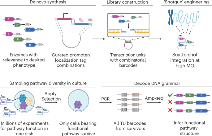
  • Decoding systemic vascular health and hypertensive disorders in pregnancy through retinal imaging and Visionary AI

    Decoding systemic vascular health and hypertensive disorders in pregnancy through retinal imaging and Visionary AI

    Main

    Hypertensive disorders of pregnancy (HDPs), including gestational hypertension (GHTN), preeclampsia, chronic hypertension (CHTN) with superimposed preeclampsia (PEC) and eclampsia, affect 2–15% of pregnancies and represent the second leading cause of maternal mortality worldwide1. HDPs increase the risk of acute maternal complications such as renal dysfunction, pulmonary edema, stroke and death2 and contribute to adverse fetal outcomes, including small for gestational age, preterm delivery and stillbirth3. Long-term, they are associated with elevated maternal risk of hypertension, coronary artery disease, stroke and vascular dementia4,5,6 and elevated offspring risk of cardiovascular and neurodevelopmental disorders7.

    Despite their burden, HDPs are typically diagnosed after 20 weeks of gestation, when symptoms such as hypertension, proteinuria or organ dysfunction become clinically apparent. Severe features, including systolic blood pressure (BP) ≥ 160 mmHg or diastolic BP ≥ 110 mmHg, thrombocytopenia and visual symptoms, guide early delivery decisions because of high maternal–fetal risk8. Among HDPs, early-onset preeclampsia (EOPE, symptoms appear before 34 weeks) tends to present with more severe complications than late-onset preeclampsia (LOPE). Notably, recent systems biology studies suggest that preeclampsia is not a single disease entity but may reflect multiple distinct biological pathways, with EOPE more frequently associated with placental dysfunction and LOPE more often associated with maternal processes9,10.

    Mechanistically, preeclampsia is believed to arise, in part, from maternal vascular inflammation and thrombosis that disrupt placental development9,11. Inflammation and thrombosis may impair deep placental invasion12 of the maternal decidua between 10 and 16 weeks of gestation and contribute to later placental injury, including placental atherosis13,14,15,16, a process that shares features with vascular pathology observed in cardiovascular disease. These early deviations from physiologic placentation precede clinical symptoms by weeks or months, underscoring the need for early biomarkers of systemic and placental vascular stress.

    From a health systems perspective, HDPs accounted for an estimated 2.18 billion USD in US healthcare costs per year (estimated in 2012), largely driven by preterm birth complications17. Their incidence has increased in subsequent years18,19,20 and pregnancies complicated by HDPs typically end approximately 3 weeks earlier than normotensive pregnancies21. Importantly, randomized trials show that early initiation of low-dose aspirin (before 16 weeks) can reduce the risk of preterm delivery with preeclampsia by up to 62%22,23 but this requires early, accurate risk identification.

    Current diagnostic criteria for preeclampsia rely on late-onset symptoms (hypertension, proteinuria and end-organ dysfunction) that usually manifest in the third trimester24. While known risk factors (for example, prior HDPs, diabetes, obesity and age) provide some predictive value, they lack individual-level accuracy25. The sFlt-1/PlGF ratio is the most validated biomarker but is primarily useful later in pregnancy and in individuals with suspected preeclampsia to aid short-term clinical assessment26. First-trimester screening tools, such as the Fetal Medicine Foundation (FMF) risk calculator27, combine clinical variables with biomarkers or ultrasound but these protocols are expensive, logistically complex and inconsistently implemented28,29. In routine practice, prevention-oriented risk stratification is often reduced to clinical risk factor assessment for aspirin eligibility, which may miss individuals with emerging vascular dysfunction while also identifying broad high-risk groups with limited precision.

    Increasing evidence suggests a link between placental vascular changes associated with preeclampsia and alterations in the retinal vasculature. Studies of women with established preeclampsia describe retinal signs resembling hypertensive retinopathy, arteriolar narrowing and choroidal changes30,31,32,33,34 and link preeclampsia to increased future risk of retinal diseases35. Further, recent evidence has identified an association between the sFlt-1/PlGF ratio and choroidal thickness as measured by optical coherence tomography (OCT)33,36. A prior postpartum study from our team (31 severe preeclampsia cases and 35 normotensive controls) demonstrated significantly increased median tortuosity in the inferotemporal retinal artery among individuals with preeclampsia37. OCT angiography has revealed that pregnant women who go on to develop placental insufficiency have significantly narrower retinal blood vessels (arterioles and venules) compared to normotensive pregnancies38. These individuals also exhibit reduced capillary density. In separate studies, women with preeclampsia had significantly lower vessel densities in both the superficial and deep capillary plexuses, including in the foveal and parafoveal regions, relative to healthy pregnant or nonpregnant controls39,40. These findings suggest a degree of capillary dropout or ‘vascular rarefaction’ in the retinas of women with preeclampsia. Retinal vessel caliber reduction and reduced perfusion density are consistent with systemic vasoconstriction and endothelial dysfunction, both hallmarks of preeclampsia pathophysiology. Importantly, these changes may be subclinical and may emerge before overt clinical diagnosis, suggesting that the maternal retina could provide a noninvasive window into systemic vascular remodeling during pregnancy.

    Initial efforts to apply AI to HDP prediction using retinal imaging have been promising but limited. The PROMPT model (preeclampsia risk factor + ophthalmic data + mean arterial pressure prediction test)41 relied heavily on clinical variables (for example, mean arterial pressure) and achieved modest image-only performance using cross-validation at a single site (area under the curve (AUC) = 0.74). Another study combining 45° retinal fundus images with clinical data reported improved accuracy but used a convolutional neural network (CNN) architecture that lacks interpretability and biological insight42. Notably, both studies were conducted in homogeneous East Asian populations, further limiting their generalizability and translational impact. Although not originally designed for preeclampsia (or any other pregnancy disorder), RETFound43 is a retinal foundation model that was validated across diverse disease classification tasks. However, direct image-level foundation-model fine-tuning may require larger numbers of outcome events than are typically available in prospective pregnancy cohorts, motivating approaches that reduce image dimensionality while preserving biologically meaningful vascular structure.

    Here we introduce Visionary AI, an end-to-end computational framework that takes as input retinal images and predicts an individual’s risk of HDPs. Unlike prior approaches that treat retinal images as opaque inputs to generic deep-learning models, Visionary AI models the retinal vasculature as a quantifiable, interpretable biological system—one that may reflect systemic endothelial and angiogenic processes occurring during placental development.

    We show across a cohort of 1,267 pregnant participants that this framework enables accurate and interpretable prediction of preeclampsia and GHTN months before clinical diagnosis. We further develop a stability-optimized model that reduces complexity and transfers to an independent New York University (NYU) validation cohort without retraining or optimization using NYU outcome labels. By benchmarking Visionary AI against the FMF risk calculator, real-world aspirin-eligibility criteria and RETFound foundation model, we evaluate whether retinal vascular modeling provides information beyond established clinical and image-level deep-learning approaches. Together, these results establish retinal vascular phenotyping as a promising new dimension of pregnancy risk assessment and position Visionary AI as an interpretable, noninvasive framework for detecting early systemic vascular remodeling before HDPs become clinically apparent.

    Results

    Cohort characteristics and study design

    We analyzed retinal imaging and clinical data from a Columbia University (CU) development cohort and an independent NYU external validation cohort.

    The CU cohort included 1,267 pregnant individuals receiving prenatal care at NewYork-Presbyterian/CU Irving Medical Center between 2021 and 2025 (Extended Data Table 1). Within the CU cohort, 55 participants developed preeclampsia (4.3%). One participant with preeclampsia was excluded from retinal image analysis because of poor image quality, yielding 54 preeclampsia cases for retinal-model analyses. Retinal images were acquired during the first, second and third trimesters using the Optos scanning laser ophthalmoscope Primary ultrawidefield imaging system.

    The independent NYU external validation cohort included 79 pregnant individuals receiving prenatal care at the Mignone Women’s Health Collaborative at NYU Langone Health between 2025 and 2026 (Extended Data Table 2). Within the cohort, 14 participants were diagnosed with preeclampsia during routine prenatal care (17.7%), representing a higher observed prevalence than the annual average prevalence of preeclampsia at NYU Langone Health (~8%). Because predictive values and precision-based metrics are sensitive to outcome prevalence, prevalence-adjusted performance estimates are reported below for both cohorts. One participant with preeclampsia was excluded from retinal image analysis because of poor image quality, yielding 13 preeclampsia cases for retinal-model analyses. NYU images were acquired during the first, second and third trimesters using the Optos California ultrawidefield imaging system.

    In both cohorts preeclampsia diagnoses were given according to 2013 American College of Obstetricians and Gynecologists (ACOG) criteria8 during prenatal care and independently reviewed by maternal–fetal medicine specialists masked to retinal imaging results. Preeclampsia cases were further categorized by severity and timing of onset, including preeclampsia with severe features (SF), preeclampsia without severe features (NSF), EOPE and LOPE; detailed definitions are provided in the Methods. Preeclampsia subtype-specific analyses were treated as descriptive evaluations of model behavior across clinical presentations rather than separately trained subtype-specific models.

    Extended Data Tables 1 and 2 summarize demographic, clinical and pregnancy-outcome characteristics for the CU and NYU cohorts. Collected variables included maternal age, height, weight, race and ethnicity, tobacco use, obstetric history, preexisting conditions, medication exposures, pregnancy complications and birth outcomes, including small for gestational age, severe small for gestational age, stillbirth, birth weight and Apgar scores.

    The CU cohort was predominantly Hispanic or Latinx, reflecting the clinical population served at the recruitment site (Supplementary Table 1). Participants who developed preeclampsia were more likely than those who did not to have a history of preeclampsia in a prior pregnancy (16.4% versus 3.8%; P = 4.1 × 10−5, chi-square test) and preexisting hypertension (18.2% versus 3.5%; P = 5.5 × 10−7, chi-square test). Participants who developed GHTN also had higher rates of obesity than normotensive population-wide (PW) controls (65% versus 33%; P = 6.5 × 10−6, chi-square test).

    The NYU cohort differed from the CU cohort in several clinically relevant respects, including race and ethnicity distribution, older maternal age, higher in vitro fertilization (IVF) prevalence and higher observed preeclampsia prevalence (Supplementary Tables 1 and 2). Among participants with race information available, the NYU cohort included a larger proportion of white and Asian participants than the CU cohort. NYU imaging was also performed using the Optos California ultrawidefield system (CU cohort used the Optos Primary ultrawidefield system) within a different clinical workflow. Together, these demographic, clinical, workflow and imaging-device differences support the use of NYU as a meaningful external validation cohort rather than a near replication of the CU development cohort.

    The Visionary AI Framework and evaluation strategy

    Visionary AI is an interpretable retinal vascular modeling framework that uses retinal images to quantify early-pregnancy microvascular structure and predict subsequent HDPs. Figure 1 summarizes the study design and computational workflow, including retinal image acquisition, vessel segmentation, vascular feature extraction and ensemble-based risk prediction.

    Fig. 1: Study design and Visionary AI computational framework.

    a, Timeline of retinal imaging and clinical outcome ascertainment. Participants were approached for ultrawidefield retinal imaging during the first, second and third trimesters. In the CU development cohort, prediction analyses used first-trimester images when available and second-trimester images only for participants without first-trimester imaging, as specified in the corresponding analyses. The NYU external validation analysis was restricted to retinal images acquired during the first trimester, between 6 and 13 weeks of gestation. Preeclampsia diagnoses were ascertained after 20 weeks of gestation according to clinical criteria. b, Central hypothesis. Retinal vascular structure in early pregnancy contains quantifiable microvascular signatures of systemic vascular dysfunction that precede clinical diagnosis of preeclampsia. c, Visionary AI pipeline. The computational workflow consists of three modules. (i) Image processing: ultrawidefield fundus images are acquired from both eyes, converted into VSIs using a designated AI model and merged when multiple images from the same eye are available to generate a more complete retinal vascular representation. (ii) Feature generation: VSIs are transformed into graph-based, geometric and topological vascular features that quantify complementary aspects of retinal microvascular architecture. (iii) Predictive modeling: semantically grouped vascular feature sets are used to train base learners and their out-of-fold predictions are integrated by a stacked metalearner to generate the final risk prediction.

    Briefly, retinal images were converted into vessel segmentation images (VSIs) using a dedicated retinal vessel segmentation AI model developed for this study. VSIs provide a binary representation of the retinal vascular tree for downstream feature extraction. When multiple images were available for a given eye, VSIs were merged to generate a more complete vascular representation for analysis. Detailed segmentation model development, image-registration and quality-control procedures are provided in the Methods.

    Visionary AI then transformed each VSI into biologically interpretable vascular representations. These included graph-based features capturing branching and connectivity, geometric features capturing vessel length, caliber, curvature, angle and tortuosity and higher-order topological features capturing vascular organization and loop structures across scales (Methods and Supplementary Note 1). Together, these feature classes were designed to summarize complementary dimensions of retinal microvascular architecture rather than treat the image as an opaque input to a generic deep-learning classifier.

    Extracted vascular features were grouped into semantically related feature sets and each feature set was used to train an independent base learner. Base-learner predictions were then integrated through a stacked ensemble framework in which out-of-fold base-learner predictions served as inputs to a metalearner. This architecture allowed the model to combine complementary vascular representations while preserving interpretability at the level of feature classes and retained base learners.

    Because preeclampsia is a relatively rare outcome, CU model development used leave-one-out cross-validation (LOOCV) to maximize training data while generating held-out predictions for each participant. To reduce the risk of information leakage, base-learner fitting and selection and metalearner training and prediction were implemented within the cross-validation framework, with out-of-fold predictions carried forward between stages, as detailed in the Methods. Model evaluation focused on both internal CU performance and external validation. Within CU, we assessed held-out cross-validated performance and the reproducibility of selected retinal vascular representations across control populations; in parallel, we evaluated model transferability in an independent NYU external validation cohort.

    Therefore, we evaluated Visionary AI across three increasingly stringent settings. First, a high-contrast analysis tested whether retinal vascular features could distinguish preeclampsia cases from a narrowly defined healthy-control group. Second, a performance-optimized CU model evaluated predictive performance across population-wide control settings within the CU development cohort. Third, to support external validation, a stability-optimized CU model was designed to prioritize reproducibility across nonoverlapping population-wide control groups rather than maximize within-site performance. This stability-optimized model used stability-based hyperparameter selection, minimum-performance and average precision (AP) variability criteria, recursive feature elimination (RFE) and feature-set deduplication to contract the candidate model space before NYU testing. The resulting model was then evaluated on the independent NYU cohort without retraining, refitting or optimization using NYU outcome labels.

    Retinal vascular features predict preeclampsia across increasingly stringent evaluation settings

    High-contrast CU analysis identifies preeclampsia-associated retinal vascular signal

    We first evaluated Visionary AI in a high-contrast CU analysis to determine whether retinal vascular features captured in early pregnancy contained detectable signals associated with subsequent preeclampsia. In this analysis, preeclampsia cases were compared to a narrowly defined healthy-control group selected to minimize medical, ocular, medication-related and pregnancy-related conditions that could independently influence retinal vascular structure. Healthy controls were drawn from singleton pregnancies without documented preexisting maternal comorbidities, ocular conditions, relevant medication exposures or pregnancy complications; detailed exclusion criteria are provided in the Methods. From 176 eligible healthy controls, 82 were selected to preserve class balance and support approximate matching on key demographic and imaging variables.

    Visionary AI distinguished participants who later developed preeclampsia from healthy controls with high apparent performance (n = 136, including 54 preeclampsia cases; AUC = 0.94, AP = 0.92, positive predictive value (PPV) = 0.85; Extended Data Fig. 1). We interpret this analysis as an initial proof of signal rather than as the primary estimate of clinical performance, as the comparison was intentionally enriched for phenotypic contrast. Therefore, we subsequently evaluated Visionary AI on broader population-wide CU control settings and on an independent NYU external validation cohort as detailed below.

    Population-wide CU analyses support preeclampsia prediction in a clinically heterogeneous obstetric population

    We next evaluated whether the retinal vascular signal identified in the high-contrast analysis persisted when preeclampsia cases were compared to broader population-wide controls from the CU cohort. Unlike the selected healthy-control analysis, these population-wide controls were drawn from the larger nonpreeclampsia obstetric population and were intended to better reflect the clinical heterogeneity encountered in prenatal care. We refer to this model as the ‘performance-optimized retinal model’, reflecting its optimization for predictive performance within the CU population-wide evaluation framework.

    Exclusions from the population-wide control pool were limited to prespecified conditions that could confound the outcome definition or preclude valid retinal-model evaluation, including multifetal gestation, HELLP syndrome, other maternal hypertensive disorders, stillbirth and unavailable or low-quality retinal images (Methods). This design retained participants with common clinical comorbidities, including CHTN, diabetes (gestational and chronic), obesity and fetal outcomes such as growth restriction, thereby providing a more heterogeneous internal evaluation than the healthy-control contrast.

    Across repeated CU population-wide control samplings, the performance-optimized retinal model maintained strong discriminative performance for preeclampsia, achieving an AUC of 0.91 ± 0.05 and an AP of 0.81 ± 0.11 across sampled control sets (Fig. 2a,b). Because this evaluation used sampled control sets rather than analyzing the full population-wide control pool at once precision–recall (PR) metrics and PPV estimates from these sampled sets should not be interpreted as real-world screening performance at the observed CU preeclampsia prevalence. Therefore, we report threshold-based operating characteristics, including prevalence-adjusted PPV and negative predictive value (NPV), in Extended Data Table 3. Together, these results show that retinal vascular features remained predictive in a broader and more clinically heterogeneous CU control population, with the modest reduction in performance relative to the high-contrast analysis likely reflecting greater biological and imaging heterogeneity.

    Fig. 2: Performance-optimized Visionary AI predicts preeclampsia in CU population-wide evaluation.

    a, ROC and PR curves for the performance-optimized Visionary AI model, the FMF risk calculator and a combined Visionary AI + FMF model within the CU population-wide evaluation framework. The analysis included 1,137 unique CU participants, including 54 preeclampsia cases. Each sampled evaluation set included 82 selected healthy controls and approximately 100 additional unique population-wide controls (Methods). In ROC plots, the diagonal line indicates no-discrimination performance (equivalent to random classification; AUC = 0.5). In PR plots, the horizontal line indicates the expected precision of a random classifier, corresponding to the prevalence of the positive class in the respective evaluation set. Shaded areas indicate 95% pointwise confidence intervals constructed using the mean ± 1.96 × s.e.m. across ten population-wide groups. Panel legends report the AUC and AP as the mean ± s.d. Visionary AI achieved higher AUC and AP than FMF. Combining Visionary AI predictions with FMF probabilities did not materially improve performance over Visionary AI alone. b, Threshold-based operating characteristics of the performance-optimized Visionary AI model across preeclampsia subtypes, based on the overall preeclampsia model. Bar plots show the AUC, PPV, NPV and TPR at the prespecified classification threshold of 0.5; the corresponding FPR was 0.08 for all subtype evaluations. Because PPV and PR metrics are prevalence dependent, the values shown reflect the sampled CU population-wide evaluation structure; prevalence-adjusted metrics standardized to a 4% preeclampsia prevalence in CU are provided in Extended Data Table 3. c, Metalearner importance of retained base learners, aggregated across folds, in the performance-optimized Visionary AI model. Base learners are annotated according to their retinal vascular categories, including vessel extension and initiation, vessel curvature and caliber, loop redundancy or resilience and vascular organization and sparsity. LR, logistic regression; RF, random forest; XGB, extreme gradient boosting.

    Combining Visionary AI with probabilities from the FMF risk calculator27, an established clinical risk prediction tool based on maternal clinical features and pregnancy-related risk factors (Methods), did not materially improve predictive performance relative to Visionary AI alone (AUC = 0.90 ± 0.06, AP = 0.80 ± 0.11). Throughout the retinal-model analyses, we accounted for first pregnancy and prior preeclampsia history as minimal obstetric-history adjustment variables (Methods); however, the primary predictive signal was derived from retinal vascular features rather than from a broader clinical risk model (Fig. 2c). These results suggest that retinal imaging features captured most of the signal relevant to preeclampsia risk in the CU population-wide analysis, with limited incremental contribution from FMF-derived clinical risk information.

    Because subtype-specific case counts were limited, analyses of SF, NSF, EOPE and LOPE were treated as post hoc stratified evaluations of the same overall preeclampsia model rather than as separately trained subtype-specific classifiers. Visionary AI, trained on all preeclampsia cases, maintained consistent predictive performance across clinical presentations, including SF (n = 38), NSF (n = 16), EOPE (n = 20) and LOPE (n = 34). At an operating point corresponding to a false positive rate (FPR) of 0.08, the true positive rate (TPR) exceeded 0.70 for each subtype (Fig. 2b). To further characterize subtype performance across a range of operating points, Supplementary Tables 3–5 report mean confusion-matrix counts and performance metrics across the ten performance-optimized population-wide control sets at thresholds targeting FPRs of up to 10%, 20% and 30%, respectively. These post hoc analyses suggest that the retinal vascular signal was not restricted to a single preeclampsia presentation, while also underscoring the need for larger cohorts to estimate subtype-specific performance more precisely.

    A stability-optimized model reduces complexity and prioritizes reproducible retinal vascular signal

    Although the performance-optimized retinal model demonstrated strong predictive performance within CU population-wide analyses, it was designed to maximize internal performance within this population. To further evaluate the robustness of the retinal vascular signal and assess whether predictive performance could be maintained under a more constrained modeling framework, we next developed a stability-optimized model designed to prioritize reproducibility across nonoverlapping population-wide control groups rather than peak performance in any single CU control setting.

    For the stability-optimized model, we used a control definition that was similar to the performance-optimized population-wide analysis but deliberately more inclusive of the clinical heterogeneity encountered in routine obstetric care. Unlike the performance-optimized model, participants with HDPs other than preeclampsia, including GHTN, were retained in the control pool rather than excluded. Furthermore, in this model, each healthy control was included only once, and the healthy-control group together with the expanded population-wide control pool, including GHTN and CHTN, was divided into five nonoverlapping control settings (Methods). Hyperparameter configurations were selected on the basis of low variability in AP and high minimum AUC across these settings, thereby favoring base learners with consistent performance across control definitions (Supplementary Fig. 1). Candidate base learners that did not meet minimum stability and performance criteria were removed before metalearner training.

    This stability-based procedure substantially reduced model complexity. The initial search space included 96 candidate base learners, representing 32 retinal vascular feature sets across three model classes. After stability-based hyperparameter selection and RFE, each leave-one-out stability-optimized model retained eight nonredundant base learners per fold. To construct the final model for each population-wide control group, we took the union of base learners selected across leave-one-out folds and retained eight nonredundant learners by prioritizing higher-importance models and removing redundant feature sets (Extended Data Fig. 2 and Methods). Thus, the model used for external validation was intentionally constrained to a small set of reproducible retinal vascular representations rather than optimized solely for maximal internal CU performance.

    Despite this reduction in model complexity, the stability-optimized model preserved predictive signal in the CU population-wide analyses, supporting the robustness of the selected retinal vascular features (Fig. 3a). Recurrent vascular feature categories and base learners, including graph-based topology, box counting, cumulative size distribution, vessel length or angle and tortuosity-related representations, were repeatedly selected and assigned high importance across population-wide settings (Fig. 3b,c and Supplementary Fig. 2). This consistency across distinct control settings suggests that model performance was driven by stable retinal microvascular representations associated with preeclampsia risk, rather than by control-set-specific patterns, fold-specific model components or unstable feature-selection artifacts.

    Fig. 3: Stability-optimized Visionary AI predicts preeclampsia in CU population-wide analyses.

    a, ROC and PR curves for the stability-optimized Visionary AI model evaluated in the CU population-wide cohort (n = 1,188; 54 preeclampsia cases). In ROC plots, the diagonal line indicates no-discrimination performance (equivalent to random classification; AUC = 0.5). In PR plots, the horizontal line indicates the expected precision of a random classifier, corresponding to the prevalence of the positive class in the respective evaluation set. Shaded areas indicate 95% pointwise confidence intervals constructed using the mean ± 1.96 × s.e.m. across five population-wide groups. Panel legends report the AUC and AP as the mean ± s.d. b, Ranked metalearner category importance across population-wide control groups. Mixed-feature base learners were excluded from the category-level analysis because they included features spanning multiple vascular categories. c, Stable selection and importance of retained base learners across CU stability-optimized population-wide models. For each population-wide control setting, RFE retained eight base learners within each leave-one-out fold. Final retained base learners were selected by prioritizing average importance across folds while removing base learners trained on redundant feature sets. The heat map shows metalearner importance for retained base learners; model classes are indicated in parentheses.

    The stability-optimized model generalizes to the independent NYU validation cohort

    We next evaluated whether the stability-optimized CU model generalized to an independent external validation cohort collected at NYU. This analysis was designed as the primary external test of the retinal vascular signal identified in the CU cohort. The NYU cohort differed from the CU development cohort in institution, population, clinical workflow and ultrawidefield imaging-device configuration and the validation analysis was restricted to retinal images during the first trimester, acquired between 6 and 13 weeks of gestation. The stability-optimized model was evaluated in NYU without retraining, refitting or hyperparameter optimization using NYU outcome labels.

    Despite these differences in site, population, imaging workflow and clinical setting, Visionary AI maintained robust predictive performance in the independent NYU validation cohort, achieving an AUC of 0.81 and an AP of 0.68 (Fig. 4a). Performance was also preserved in differential-diagnosis analyses distinguishing preeclampsia from other HDPs, including GHTN and CHTN, as well as in subgroup analyses stratified by demographic characteristics, clinical risk factors and quality-control metrics (Extended Data Fig. 3 and Supplementary Figs. 3–5).

    Fig. 4: Stability-optimized Visionary AI performance predicting preeclampsia on NYU external validation cohort.

    a,b, ROC (left) and PR (right) curves for the stability-optimized model evaluated on the independent NYU external validation cohort (a; n = 66, 13 preeclampsia cases) and ‘the aspirin-recommended subgroup analysis’ (b; n = 33, eight preeclampsia cases). In ROC plots, the diagonal line indicates no-discrimination performance (equivalent to random classification; AUC = 0.5). In PR plots, the horizontal line indicates the expected precision of a random classifier, corresponding to the prevalence of the positive class in the respective evaluation set.

    Unlike the CU population-wide analyses, the NYU validation did not rely on repeated or balanced sampled control sets. Thus, threshold-based PPV and NPV calculated directly from this cohort reflect the observed preeclampsia prevalence in the NYU validation set. At a stringent operating point, Visionary AI achieved an FPR of 0.02, TPR of 0.46, PPV of 0.86 and NPV of 0.88; at a less stringent operating point, Visionary AI achieved an FPR of 0.13, TPR of 0.69, PPV of 0.56 and NPV of 0.92 (Extended Data Table 4). Because the observed preeclampsia prevalence in the NYU validation cohort was higher than the annual average prevalence at NYU Langone Health (approximately 8%), we additionally report prevalence-adjusted PPV and NPV using the institutional annual prevalence estimate. Under this prevalence-adjusted setting, the stringent operating point corresponded to an estimated PPV of 0.68 and NPV 0.95, whereas the less stringent operating point corresponded to an estimated PPV of 0.31 and NPV of 0.97 (Extended Data Table 4). The preservation of predictive signal in an independent, early-pregnancy validation cohort supports the transferability of the retinal vascular features selected by the stability-optimized CU model.

    Together, these findings show that the constrained stability-optimized model retained predictive signal beyond the CU development setting. The successful transfer of the stability-optimized model across sites, clinical workflows, populations and imaging-device configurations supports the interpretation that Visionary AI captures reproducible retinal microvascular signatures associated with preeclampsia risk rather than CU-specific control-set artifacts or unstable ensemble behavior.

    Visionary AI complements established clinical risk-stratification approaches

    We next evaluated Visionary AI against established clinical risk-stratification approaches for preeclampsia. To provide a clinically relevant benchmark and avoid potential bias associated with locally trained or modified FMF implementations, we used the official FMF risk calculator portal directly for the independent NYU validation cohort. This analysis used the available maternal demographic, clinical and family-history variables required by the FMF first-trimester risk assessment framework, including maternal age, height, weight, racial origin, CHTN, type 1 diabetes, smoking status, systemic lupus erythematosus, method of conception, obstetric history and family history of preeclampsia (Methods).

    In the NYU external validation cohort, Visionary AI outperformed FMF across both receiver operating characteristic (ROC) and PR analyses, achieving an AUC of 0.81 and an AP of 0.68, compared to FMF AUC of 0.73 and AP of 0.50 (Fig. 4a). At clinically relevant low-FPR operating points, Visionary AI also achieved higher sensitivity and precision than FMF. At a stringent threshold (FPR of 0.02), Visionary AI achieved a TPR of 0.46 and prevalence-adjusted PPV of 0.68. At a less stringent threshold, Visionary AI achieved an FPR of 0.13, TPR of 0.69 and prevalence-adjusted PPV of 0.31, compared to the FMF FPR of 0.13, TPR of 0.38 and prevalence-adjusted PPV of 0.20 (Extended Data Table 4). Bootstrap resampling of the NYU cohort, stratified by outcome to preserve the observed case prevalence, yielded consistent performance estimates, quantified uncertainty around the ROC, PR and threshold-based metrics and showed that Visionary AI consistently outperformed FMF (Supplementary Table 6).

    We also compared Visionary AI to the clinical risk-stratification approach used at NYU to guide aspirin eligibility on the basis of ACOG guidelines at approximately 12 weeks of gestation. This benchmark reflects routine prenatal-care decision making on the basis of clinical risk factors, including IVF, maternal age over 35 years and BMI over 30 (Methods). In the NYU cohort, aspirin eligibility identified preeclampsia cases with a TPR of 0.62 but at a substantially higher FPR of 0.47 and lower prevalence-adjusted PPV of 0.1. In contrast, Visionary AI achieved a TPR of 0.69 at a FPR of 0.13 with a prevalence-adjusted PPV of 0.31. These results support the potential of Visionary AI to provide retinal vascular information that is complementary to current clinical risk-factor-based screening and prevention strategies.

    As an additional sensitivity analysis, we evaluated the stability-optimized Visionary AI model within the subset of NYU participants who were recommended aspirin during pregnancy, a clinically enriched group expected to have elevated baseline risk on the basis of routine obstetric assessment (n = 33, eight preeclampsia cases). In this aspirin-recommended subgroup, Visionary AI maintained strong predictive performance, achieving an AUC of 0.95 and an AP of 0.85, compared to the FMF AUC of 0.76 and AP of 0.65 (Fig. 4b). Combining Visionary AI with FMF probabilities did not improve performance (AUC = 0.78, AP = 0.67), consistent with the broader analysis. Although this subgroup analysis is limited by sample size, the preservation of strong retinal-model performance among aspirin-recommended individuals suggests that Visionary AI captures retinal vascular information not fully represented by the clinical risk factors used to guide aspirin recommendation.

    Because the CU cohort lacked some FMF variables, including family history of preeclampsia and a direct systemic lupus erythematosus variable, CU FMF comparisons were treated as secondary benchmarking analyses and interpreted with caution. Across both CU performance-optimized and stability-optimized analyses, Visionary AI showed stronger performance than FMF-derived clinical risk estimates; however, the NYU analysis represents the most complete and clinically relevant FMF comparison in the revised manuscript. Together, these results suggest that Visionary AI captures retinal vascular information that is not fully represented by existing clinical risk-stratification tools.

    Visionary AI outperforms direct image-level RETFound foundation model and Inception-ResNet-v2 in limited-event clinical cohorts

    We next benchmarked Visionary AI against two image-based deep-learning approaches: RETFound, a retinal foundation model, and Inception-ResNet-v2, a CNN. Both baselines were trained on the CU development cohort using participant-level LOOCV. In each iteration, all retinal images from the held-out participant were excluded together from model training, preprocessing decisions and model selection, thereby preventing image-level leakage across participants. Image-level probabilities were averaged across all available images from each participant to obtain participant-level predictions for evaluation.

    RETFound was initialized using publicly available pretrained weights and fine-tuned for preeclampsia prediction for up to 25 epochs using the developers’ publicly available scripts and default fine-tuning parameters. Inception-ResNet-v2 was evaluated as a transfer-learning CNN baseline for up to 25 epochs. The pretrained convolutional backbone was held fixed and only a new classification layer was trained; thus, this analysis assessed a classification head trained on fixed pretrained image representations rather than full end-to-end fine-tuning. Training used weighted cross-entropy loss, with weights of 1 for controls and 4 for cases to account for the approximately 20% case prevalence in the training data.

    For external evaluation, the CU-trained RETFound and Inception-ResNet-v2 models were applied to the independent NYU cohort without using NYU outcomes for model fitting, fine-tuning, hyperparameter or epoch selection or calibration. Under these training and evaluation configurations, both image-level baselines performed near chance in the NYU cohort (Supplementary Figs. 6 and 7), whereas Visionary AI maintained strong predictive performance in external validation. We interpret these findings cautiously, as deep-learning models may require substantially larger numbers of outcome events for effective task-specific training or fine-tuning. The results therefore do not establish that Visionary AI is generally superior to deep learning. Rather, within the evaluated sample sizes and training configurations, RETFound and Inception-ResNet-v2 did not match Visionary AI’s predictive performance. These findings are consistent with the possibility that lower-dimensional, biologically informed representations of retinal vascular topology, geometry and network organization may be advantageous in clinical cohorts with limited numbers of outcome events.

    Stable retinal vascular signatures support biological interpretability of Visionary AI

    Having established that Visionary AI predicted preeclampsia across CU population-wide analyses, generalized to an independent NYU validation cohort and outperformed clinical and deep-learning benchmarks, we next examined the retinal vascular representations that contributed to model predictions. Because Visionary AI is built from predefined vascular feature sets rather than opaque image-level embeddings, model interpretation could be performed across retained base learners and aggregated broader vascular categories.

    Across the performance-optimized and stability-optimized CU models, importance analyses converged on recurring retinal vascular representations related to graph topology, geometry, nesting tree (that is, summarizes the hierarchical organization of loops and bifurcations) and complexity (Fig. 3b and Supplementary Fig. 8). In the performance-optimized model, graph topology and complexity-related base learners showed the highest importance, with informative base learners including box counting, fractal organization, graph topology and vessel branching angles (Fig. 2c). In the stability-optimized model, recurrent base learners, including box counting, graph-based topology, cumulative size distribution, vessel length or angle and tortuosity-related features, were repeatedly selected across nonoverlapping population-wide control groups and assigned high importance (Fig. 3c). The features within base learners were also consistently assigned high importance across control populations, illustrating the stability of vascular trait importance within base learners across population-wide control groups and folds (Supplementary Figs. 9–11). For example, the vascular traits quantified in the ‘cumulative size distribution of loops’ base learner were consistently ranked high across folds and population-wide control settings (Supplementary Fig. 9). This consistency across models and control definitions suggests that Visionary AI performance is driven by a reproducible subset of retinal vascular representations rather than control group specific feature selection, artifacts or a narrow control-selection strategy (Supplementary Note 2).

    To further evaluate the biological relevance of these model-derived signatures, we performed model-independent univariate analyses of representative retinal vascular features. These analyses identified preeclampsia-associated differences in features related to vessel branching, topological length, tortuosity, vessel thickness, fractal organization, loop count and vascular asymmetry (Fig. 5 and Supplementary Note 3). Collectively, these features point to alterations in retinal vascular density, branching organization, vessel extension, curvature and network redundancy—properties that are consistent with microvascular remodeling and systemic endothelial dysfunction in HDPs.

    Fig. 5: Preeclampsia-associated features capture clinically relevant vascular properties.

    Columns show selected retinal features from four feature categories used to construct base learners: graph topology, geometry, nesting tree and complexity. a, For each feature, boxplots compare preeclampsia cases (n = 54), healthy controls (n = 82) and population-wide controls (n = 1,134). Boxes show the IQR, center lines indicate the median, whiskers extend to the most extreme values within 1.5× the IQR and overlaid points represent individual participants. b, Schematics illustrate how each feature differs between healthy and preeclampsia-associated vascular patterns. c, Corresponding vascular properties represented by the features are shown. Branch count quantifies the number of branch nodes (black circles in b) and differs between preeclampsia cases and healthy controls (P = 0.04). Mean weighted inferior topological length shift captures differences in branch extension based on the number and weighting of nodes between the vascular root and terminal tips and differs between preeclampsia cases and healthy controls (P = 0.02) and population-wide controls (P = 0.01). Total squared-curvature tortuosity quantifies vessel curvature along the vascular path and differs between preeclampsia cases and healthy controls (P = 0.01). Loop count quantifies redundant or interconnected paths within the vascular network and differs between preeclampsia cases and healthy controls (P = 0.007). Box counting captures vascular coverage and spatial organization using features derived by partitioning the image into a grid and identifying boxes that contain vessels. In b (right), boxes containing vessels are filled, whereas boxes without vessels remain unfilled. Box counting differs between preeclampsia cases and healthy controls (P = 0.002) and population-wide controls (P = 7.04 × 10⁻6). P values were calculated using a two-sided Mann–Whitney U-test. *P < 0.05, **P < 0.01 and ***P < 0.001. HC, healthy controls.

    These analyses should be interpreted as hypothesis generating rather than causal. Nevertheless, the combination of recurrent base-learner selection, consistent base-learner importance, stability across population-wide control groups and model-independent univariate differences supports the biological interpretability of Visionary AI. Together, these results suggest that preeclampsia risk is associated with early alterations in retinal microvascular topology, geometry and network organization that can be detected before clinical diagnosis.

    Visionary AI generalizability across GHTN and preexisting hypertension

    Lastly, we evaluated the ability of the Visionary AI framework to predict additional hypertensive disorders, specifically GHTN and CHTN diagnosed before pregnancy. Although both GHTN and preeclampsia are thought to originate in placental dysfunction44, we hypothesized that they give rise to distinct retinal vascular signatures detectable in first-trimester images. Specifically, we expect that preeclampsia and GHTN each produce unique patterns of microvascular remodeling, with preeclampsia potentially exhibiting more spatially extensive alterations. These clinical phenotypes also differ in their comorbidities; participants who developed GHTN had significantly higher rates of obesity (65% versus 33%; P = 6.5 × 10−6, chi-square test), while those who developed preeclampsia had higher rates of CHTN (18.2% versus 3.5%; P = 5.5 × 10−7, chi-square test).

    To this end, we used both the performance and stability-optimized model architectures to assess our approach’s generalizability in distinguishing GHTN (49 cases) and CHTN (61 cases, excluding subjects with superimposed preeclampsia). The performance-optimized model achieved an AUC of 0.91 ± 0.05 and an AP of 0.83 ± 0.07 for GHTN (n = 1,132, including 49 GHTN cases) and an AUC of 0.90 ± 0.06 and an AP of 0.79 ± 0.12 for CHTN (n = 1,106, including 61 CHTN cases). The stability-optimized models were able to predict GHTN with an AUC of 0.80 ± 0.05 and AP of 0.50 ± 0.09 (n = 1,138, including 49 GHTN cases) and CHTN with an AUC of 0.78 ± 0.02 and AP of 0.53 ± 0.04 (n = 1,143, including 61 CHTN cases) (Fig. 6a). On the NYU external validation set GHTN (n = 7) was predicted with an AUC of 0.67, AP of 0.53, and PPV of 0.50 with a TPR of 0.43 at a 0.05 FPR (Fig. 6b). We could not evaluate performance for CHTN at NYU as there were only three cases.

    Fig. 6: GHTN and CHTN stability-optimized Visionary AI model performance.

    a, ROC and PR curves for stability-optimized Visionary AI models predicting GHTN and CHTN in the CU population-wide evaluation framework (GHTN: n = 1,138, including 49 cases; CHTN: n = 1,143, including 61 cases, excluding individuals with superimposed preeclampsia) (top) and for the GHTN model in the NYU external validation cohort (n = 66, including seven cases (bottom). Shaded areas indicate 95% pointwise confidence intervals constructed using the mean ± 1.96 × s.e.m. across five population-wide groups. Panel legends report the AUC and AP as the mean ± s.d.; the NYU AUC and AP are reported as single-cohort estimates. b, Metalearner importance of retained base learners in the stability-optimized GHTN model across the five CU population-wide control groups. Colors denote the corresponding retinal vascular categories. The corresponding analysis for CHTN is shown in Extended Data Fig. 4.

    Both the GHTN and CHTN metalearner base-learner importances included superior vessel-thickness shift (thickness of vessels at the top of the eye relative to healthy controls) and topological length (number of vessel branching points) related base learners in their top three (Fig. 6b and Extended Data Fig. 4), suggesting that both modes of hypertension may contribute to abnormal vessel-thickness distributions in the retinal vasculature, as well as irregular branching patterns. Nesting number and tree base learners were also recurrent for both models, being selected across all five population-wide control groups for GHTN and four of five population-wide control groups for CHTN, suggesting an irregular structure in the loopiness or redundancy of the vasculature. Furthermore, while the GHTN model gives greater importance to topological data analysis (TDA) flooding, the CHTN model places more weight on TDA outward, indicating that these hypertensive disorders may differ in their vascular organization. Taken together, these differences indicate a simplification of hierarchical vascular organization in GHTN and CHTN, pointing to localized changes, whereas preeclampsia had greater sparsity and disorganization on a global level with the increases in tortuosity and decrease in the number of loops indicating the loss of structural regularity (Figs. 3c and 5). These results align with univariate differences between CHTN and GHTN from population-wide and healthy controls. For example, in both GHTN and CHTN, the mean weighted nesting ratio (a measure of loop asymmetry) was reduced compared to population-wide controls, indicating a simplification of hierarchical vascular organization (Extended Data Fig. 5 and Supplementary Note 3).

    Overall, our model demonstrates strong predictive performance for both conditions, supporting the notion that retinal imaging can detect early, subclinical vascular changes in high-risk pregnancies. The differences in retinal topology may reflect the divergent timing, severity or underlying mechanisms of these HDPs.

    Discussion

    Visionary AI detects retinal vascular signatures of HDPs from ultrawidefield retinal images, enabling prediction well before clinical symptoms emerge. By quantifying early retinal microvascular patterns associated with later diagnosed preeclampsia and related hypertensive disorders, Visionary AI offers a biologically grounded, interpretable and scalable framework for early risk stratification across diverse obstetric populations.

    A central advance of this work is the use of graph-based retinal vascular modeling to capture microvascular organization, including topology, vessel geometry, network complexity and hierarchical structure. These representations were predictive in the development cohort and transferred to an independent validation cohort without retraining or optimization using outcome labels. This cross-cohort transfer is particularly important, as the two cohorts differed in population, clinical workflow and imaging-device configuration, providing an initial test of robustness across real-world sources of variation.

    Another key advance of Visionary AI is its interpretable framework. The retinal features identified by Visionary AI are biologically plausible in the context of preeclampsia and related hypertensive disorders. Preeclampsia is characterized by systemic endothelial dysfunction, altered vascular tone, antiangiogenic signaling and microvascular injury. The retinal signatures detected here, involving altered vascular topology, branching structure, tortuosity, vessel caliber, loop organization and asymmetry, are consistent with early vascular simplification and reduced network resilience.

    These retinal signatures mirror vascular patterns reported in established preeclampsia and other hypertensive states40,45, including reduced vessel density, lower perfusion, diminished branching complexity and increased vascular asymmetry. Because these analyses are based on predictive feature attribution and univariate associations, they should be interpreted as hypothesis generating rather than causal evidence.

    Visionary AI captures early signs of vascular simplification, a hallmark of preeclampsia, consistent with two complementary pathological processes: capillary network rarefaction40,45 (loss of small vessels, reduced density and impaired branching complexity) and arteriolar wall thickening (hypertrophic remodeling that narrows luminal diameter and increases resistance)46. These processes jointly contribute to reduced network redundancy, lower perfusion and heightened susceptibility to ischemic injury12,14,47. Our topological metrics, including changes in loop structure, asymmetry and branching organization, are consistent with early deviations in vascular organization and network resilience. Inferior retinal differences in feature importance further align with known variations in regional blood flow48. The fact that Visionary AI identifies these shifts early in gestation underscores the system-wide vascular impairment characteristic of HDPs and provides potential mechanistic insight into disease pathways.

    We benchmarked Visionary AI against established clinical risk-stratification approaches and direct image-level deep-learning methods. In the NYU external validation cohort, Visionary AI outperformed the official FMF risk calculator, an established clinical risk prediction tool based on maternal clinical features and pregnancy-related risk factors. We also compared Visionary AI to the clinical risk-stratification approach used at NYU to guide aspirin eligibility at approximately 12 weeks of gestation. This comparison is clinically important because aspirin eligibility reflects the current prevention-oriented workflow; individuals identified as higher risk on the basis of routine obstetric risk factors are recommended low-dose aspirin. Visionary AI achieved higher sensitivity and precision at lower FPRs than aspirin eligibility alone, suggesting that retinal vascular features capture risk information not fully represented by standard clinical criteria. In an additional aspirin-recommended subgroup, Visionary AI maintained strong performance despite enrichment for individuals already identified as higher risk by routine clinical assessment, further supporting its potential to refine risk stratification within clinically high-risk groups. Together, these analyses suggest that Visionary AI provides complementary retinal microvascular information beyond both FMF-based risk estimation and ACOG-recommended aspirin-eligibility criteria.

    We also compared Visionary AI to two deep-learning models: RETFound, a retinal foundation model, and Inception-ResNet-v2, a CNN. Both deep-learning approaches performed near chance on the CU development cohort and the independent NYU validation cohort, whereas Visionary AI had strong performance and preserved predictive signal on the external validation cohort. This comparison should be interpreted cautiously, because end-to-end deep-learning models may require substantially larger numbers of outcome events for effective task-specific fine-tuning. Nevertheless, these results support the rationale for Visionary AI’s feature-based design; by converting retinal images into biologically meaningful vascular graph topology, geometry, nesting-tree and organization features, Visionary AI reduces the dimensionality of the prediction problem and may be better suited to limited-event pregnancy cohorts than direct image-level fine-tuning.

    Visionary AI offers a fast, noninvasive and cost-effective screening strategy suitable for both high-resource and low-resource settings. Retinal fundus imaging requires no laboratory infrastructure, takes less than 2 min to perform and can be operated by nonspecialists. As our computational pipeline is automated and does not require manual image grading, it eliminates subjectivity and reduces implementation barriers. Visionary AI may provide value as a retinal microvascular adjunct to existing obstetric risk assessment by capturing biological information not fully represented by clinical risk factors, FMF-based prediction or aspirin-eligibility criteria. In practice, this could support earlier and more refined risk stratification, including identification of individuals who may benefit from intensified surveillance, preventive interventions or referral pathways. Additional prospective studies will be needed to determine whether Visionary AI is best deployed as a standalone screening tool, as part of a multimodal model with established clinical and biomarker-based approaches or as a second-line test to refine risk among individuals already classified as clinically high risk. These studies will also be essential to define calibration, optimal operating thresholds, clinical utility, workflow integration and feasibility across diverse healthcare settings.

    Several limitations warrant consideration. Although our prospective CU development cohort was large for imaging-based pregnancy research, the absolute number of preeclampsia cases was modest because of low baseline prevalence. The addition of the NYU cohort provides independent external validation across site, population, clinical workflow and imaging-device configuration; however, the validation cohort remains modest in size and has a higher observed preeclampsia prevalence than the annual institutional average. Therefore, we report prevalence-adjusted PPV and NPV but larger prospective validation cohorts will be needed to estimate screening performance, calibration and decision thresholds more precisely across different baseline-risk settings.

    Additional limitations include the relatively small number of cases available for subtype-specific analyses, including EOPE and NSF. These analyses were, therefore, treated as post hoc stratified evaluations of a model trained on overall preeclampsia rather than independently trained subtype-specific classifiers. Although the stability-optimized model reduced complexity and transferred to NYU without retraining, the current study remains limited to two US academic medical centers. Importantly, the CU and NYU cohorts already differed in imaging device, acquisition workflow, race and ethnicity distribution and comorbidity profiles, providing an initial test of robustness across these sources of variation. Future studies should extend this validation to larger and more geographically diverse populations, additional healthcare systems, broader baseline-risk settings and lower-cost retinal imaging devices to determine how well the retinal vascular signal transfers across implementation contexts.

    Future and ongoing work includes multisite international validation and integration with circulating biomarkers and placental pathology for deeper mechanistic insight. Together, these efforts will determine how Visionary AI can be integrated into early pregnancy care to improve risk stratification and reduce the burden of HDPs.

    Methods

    Study design, ethics and participants

    This prospective study was approved by the Institutional Review Boards of CU and NYU and adhered to the tenets of the Declaration of Helsinki. Informed consent was obtained from every participant before enrollment. The study was designed to evaluate whether retinal vascular features captured during early pregnancy could predict subsequent HDPs. CU served as the development cohort, and NYU served as an independent external validation cohort.

    CU development cohort

    Pregnant individuals receiving prenatal care at NewYork-Presbyterian/CU Irving Medical Center between 2021 and 2025 were enrolled in the CU development cohort (n = 1,267). Eligible participants were at least 18 years of age, able to provide informed consent and could be enrolled through the second trimester of pregnancy.

    Maternal demographic and clinical data were extracted from the electronic health record, including age, race, ethnicity, obstetric history, medical history, medication exposures, laboratory values and pregnancy-related diagnoses (that is, gestational diabetes mellitus and HDPs). Delivery outcomes were also recorded, including birth weight, small for gestational age, severe small for gestational age, stillbirth and Apgar scores.

    Retinal images were obtained from each eye by trained research technicians using the Optos ultrawidefield Primary scanning laser ophthalmoscope, which captures 200° images covering approximately 80% of the retina. Images were acquired during first-trimester, second-trimester and third-trimester study visits when available. Because the primary objective was early prediction before clinical diagnosis, CU model development analyses used first-trimester images when available. For participants without first-trimester imaging, second-trimester images obtained before 20 weeks of gestation were used. History of ocular conditions and prior ocular surgery was captured and used to determine imaging-related exclusions as described below.

    NYU external validation cohort

    Pregnant individuals receiving prenatal care at the Mignone Women’s Health Collaborative at NYU Langone Health between 2025 and 2026 were enrolled in the NYU external validation cohort (n = 79). Eligible participants were at least 18 years of age and able to provide informed consent. Maternal demographic, clinical and pregnancy-outcome data were extracted from the electronic health record using the same general categories as in the CU cohort.

    Retinal images were obtained from each eye by trained research technicians using the Optos ultrawidefield California scanning laser ophthalmoscope, which also captures 200° images covering approximately 80% of the retina. The NYU cohort differed from the CU cohort in clinical workflow, imaging-device configuration, race and ethnicity distribution and comorbidity profile. For the external validation analysis, only retinal images acquired during the first trimester, until 13 weeks of gestation were used. Thus, the NYU validation analysis provided an early-pregnancy external test of the CU-trained model under a different site, population, imaging workflow and device configuration.

    Extended Data Tables 1 and 2 summarize demographic, clinical and pregnancy-outcome characteristics for the CU and NYU cohorts.

    Clinical outcomes and case definitions

    In both cohorts, HDPs were diagnosed by participants’ obstetric clinicians during routine prenatal care and extracted from the electronic health record. Preeclampsia was defined according to the 2013 American College of Obstetricians and Gynecologists criteria8. GHTN was defined as new-onset hypertension after 20 weeks of gestation without diagnostic criteria for preeclampsia. CHTN was defined as hypertension present before pregnancy or diagnosed before 20 weeks of gestation.

    Preeclampsia cases were further classified by disease severity and timing of onset. SF was defined as preeclampsia accompanied by at least one severe clinical feature, including severe-range BP (systolic BP ≥ 160 mmHg or diastolic BP ≥ 110 mmHg on two occasions more than 4 h apart), thrombocytopenia, impaired liver function, renal insufficiency, pulmonary edema or new-onset neurologic symptoms8. NSF met diagnostic criteria for preeclampsia but did not meet criteria for severe features (systolic BP ≥ 140 mmHg or diastolic BP ≥ 90 mmHg on two occasions that were at least 4 h apart, accompanied by either proteinuria or mild signs of maternal organ dysfunction)8. EOPE was defined as symptoms at or before 34 weeks of gestation and LOPE was defined as symptoms after 34 weeks of gestation.

    In the CU development cohort, 55 participants were diagnosed with preeclampsia (corresponding to 4.3% observed preeclampsia prevalence), including 38 with severe features and 17 without severe features. In total, 20 cases were classified as EOPE and 35 were classified as LOPE. All CU preeclampsia cases were independently reviewed by a maternal–fetal medicine specialist who were masked to retinal imaging results. One CU participant with preeclampsia was excluded from retinal-model analyses because of poor retinal image quality; therefore, retinal-model analyses included 54 CU preeclampsia cases where indicated.

    In the NYU external validation cohort, 14 participants were diagnosed with preeclampsia, corresponding to an observed validation cohort preeclampsia prevalence of approximately 17.7%. Preeclampsia cases included nine with severe features and five without severe features; one case was classified as EOPE and 13 cases were classified as LOPE. All NYU preeclampsia cases were independently reviewed by a maternal–fetal medicine specialist who was masked to retinal imaging results. One NYU participant with preeclampsia was excluded from the retinal-model evaluation analyses because of poor retinal image quality; therefore, retinal-model analyses included 13 preeclampsia cases were indicated.

    Birth outcomes were extracted from the electronic health record, including gestational age at delivery, birth weight, small for gestational age, severe small for gestational age, stillbirth and Apgar scores. Small for gestational age was defined as birth weight below the tenth percentile for gestational age and severe small for gestational age was defined as birth weight below the third percentile.

    Retinal image acquisition and preprocessing

    Ultrawidefield retinal images were acquired by trained research technicians at each study site. In the CU development cohort, images were acquired using the Optos ultrawidefield Primary scanning laser ophthalmoscope. In the NYU external validation cohort, images were acquired using the Optos ultrawidefield California scanning laser ophthalmoscope. Both systems capture 200° retinal images covering approximately 80% of the retina. After image-level preprocessing and quality control, the analytic retinal image dataset included 4,361 images in the CU and NYU cohorts.

    For the CU development analyses, retinal images acquired during the first trimester were used when available. For participants without first-trimester imaging, second-trimester images obtained before 20 weeks of gestation were used. This approach was selected to maximize early-pregnancy sample size while preserving the presymptomatic prediction framework. In contrast, the NYU external validation analysis was restricted to retinal images acquired until 13 weeks of gestation, only during the first trimester.

    Artifact mitigation began at image acquisition. During clinical imaging, imagers were instructed to acquire multiple images when eyelashes, eyelids, shadows, positioning differences or other localized artifacts were observed. This multi-image acquisition strategy allowed vascular regions obscured in one image to be recovered from another image of the same eye during VSI generation and merging, reducing sensitivity to localized artifacts and limiting reliance on manual exclusion of lower-quality images.

    Before vessel segmentation, retinal images were standardized to support consistent downstream processing. Each image was then cropped using a standardized elliptical mask to remove nonretinal regions and peripheral artifacts outside the retinal field of view, including eyelashes, eyelids and acquisition-related obstructions. This preprocessing step was applied programmatically and uniformly across images before AI-based vessel segmentation. The elliptical mask was 3,904 × 3,008 pixels and captured approximately 50% of the image where the majority of the retinal vasculature is captured. Images were rescaled to a uniform zoom level and resized to 912 × 912 pixels.

    Images with inadequate quality for vessel segmentation or downstream feature extraction were excluded according to prespecified quality-control procedures described below. History of ocular conditions or prior ocular surgery was also captured and used to guide image-level or participant-level exclusions where relevant.

    AI-based vessel segmentation and VSI generation

    Preprocessed ultrawidefield retinal images were converted into VSIs using a dedicated retinal vessel segmentation AI model developed for this study. VSIs provide binary representations of the retinal vascular tree and serve as the input for downstream vascular feature extraction.

    The segmentation model was inspired by retinal vessel generative adversarial network (RV-GAN) architectures and used a U-Net-based generator designed to capture both large-scale vascular structure and fine vessel detail49. The RV-GAN model was initially trained using publicly available 45° color fundus-image datasets paired with expert-annotated vessel segmentation maps50,51,52,53,54. It was then fine-tuned on a curated set of 20 ultrawidefield retinal images from the study cohort with corresponding hand-annotated vessel maps. These ultrawidefield vessel maps were reviewed by a retinal specialist to ensure anatomical plausibility and segmentation quality.

    The segmentation model generated vessel-probability maps, in which each pixel was assigned a probability of representing retinal vasculature. Probability maps were binarized using a threshold of 0.3 to preserve fine vascular detail and small disconnected components were removed during postprocessing. The resulting VSIs were used for downstream VSI merging and feature extraction.

    When multiple images were available from the same eye, VSIs were merged to generate a more complete representation of the retinal vasculature and to recover regions obscured by localized artifacts in individual images (Extended Data Fig. 6). VSI merging was performed sequentially at the eye level. First, oriented fast rotated BRIEF (ORB) keypoint detection and descriptor matching were used to identify corresponding vascular structures across VSIs. A homography transformation was then estimated using random sample consensus to achieve coarse alignment while reducing the influence of mismatched keypoints. Next, a gradient-descent image-registration algorithm was used to identify the local transformation that maximized vessel overlap between the two VSIs being merged. This deformable registration step locally adjusted the images to account for nonlinear differences in image acquisition and retinal geometry. When more than two VSIs were available for the same eye, images were merged sequentially according to acquisition order.

    After eye-level VSI generation, vascular features were extracted independently from the right and left eyes and when both were available averaged to generate participant-level feature values. One-eye imaging data were retained when image quality was sufficient for vessel segmentation and downstream feature extraction. In the CU cohort, 29 subjects only had data for one eye, while two subjects had data for only one eye in the NYU cohort.

    Image and VSI quality control and analytic image or VSI exclusions

    Image and VSI quality were evaluated using three complementary metrics designed to capture vascular completeness and common acquisition artifacts: vessel-density score, eyelash score and artifact score (Supplementary Fig. 12 and Supplementary Note 4). These metrics were used to assess whether retinal images and derived VSIs were suitable for downstream vascular feature extraction and model evaluation.

    The vessel-density score was calculated from each VSI to quantify the spatial completeness of the detected retinal vasculature. Each VSI was divided into a 12 × 12 grid and the proportion of grid squares containing vessel pixels above a prespecified threshold was calculated. A grid square was considered vessel-containing if vessel pixels exceeded 1% of the square. This score captured incomplete vascular coverage that could arise from poor image quality, obstruction or segmentation failure.

    The eyelash score was generated using an ordinal image-quality classifier trained to identify eyelash obstruction in fundus images. Images were assigned an ordinal score corresponding to no, mild, moderate or severe eyelash obstruction. This metric was used to quantify localized obscuration that could affect vessel visibility and downstream feature extraction.

    The artifact score was generated using a binary classifier trained to identify acquisition-related artifacts, including machine artifacts, shadows, eyelids and other image-quality defects that could interfere with segmentation or vascular feature extraction. Images assigned high artifact burden were reviewed according to prespecified quality-control criteria.

    Quality-control metrics were evaluated at the image, eye and participant levels.

    When multiple images were available for the same eye, localized artifacts in individual images were mitigated through VSI merging, as described above. Images or participant-level vascular representations were excluded from retinal-model analyses only when image quality was insufficient for reliable vessel segmentation or downstream feature extraction, according to prespecified segmentation quality criteria. These criteria included sparse vessel segmentation, defined by a vessel-density score < 0.25, and additional segmentation quality failures, described in Supplementary Note 5. Participants were excluded only when adequate vascular representations could not be obtained from either eye. Using these criteria, four participants were excluded from the performance-optimized CU analysis, six from the stability-optimized CU analysis with expanded controls and 13 from the NYU cohort. Sensitivity analyses evaluating robustness to image-quality variation and single-eye availability are described under model evaluation procedures, with detailed results provided in Supplementary Note 5.

    Retinal vascular feature generation

    Retinal vascular features were generated from participant-level VSIs. Feature extraction was designed to quantify complementary dimensions of retinal microvascular architecture, including graph topology, vessel geometry, vascular complexity and spatial organization and hierarchical loop structure (nesting tree). Detailed feature definitions are provided in Supplementary Note 1.

    VSIs were first converted into graph-based representations of the retinal vascular tree. Binary vessel maps were skeletonized and nodes were assigned to vessel bifurcations and terminal points. Edges represented vessel segments connecting adjacent nodes. From these graphs, we extracted features describing branching architecture and network connectivity, including numbers of nodes, bifurcation points, terminal points, connected components, internode distances and topological length. Topological length was calculated as a graph-based measure of hierarchical vessel depth, with both weighted and unweighted versions computed, and was evaluated separately in superior, inferior and whole-retina regions when applicable.

    Geometric features were extracted to quantify vessel shape, caliber and curvature. These included vessel-length and vessel-density measures, vessel-thickness features and multiple tortuosity measures. Tortuosity features summarized deviations from a straight vessel path using complementary metrics, including sinuosity, inflection-based tortuosity, curvature-based tortuosity and tortuosity density.

    To capture higher-order vascular complexity and spatial organization, we extracted box-counting, fractal and TDA features. Box-counting features quantified how retinal vessels occupied space across scales and dimensionality of high-dimensional box-counting outputs was reduced using principal component analysis before model training. TDA was used to quantify connected components and loops across multiple filtrations, including radial and distance-based filtrations. Persistence diagrams were converted into vectorized representations suitable for downstream predictive modeling, with principal component analysis used where appropriate to reduce dimensionality.

    We also extracted nesting-tree features to quantify the hierarchical organization of vascular loops and bifurcations. These features summarized loop count, loop organization, asymmetry and redundancy of the vascular network, providing complementary information about network resilience and hierarchical structure.

    For selected feature classes, distributional-shift features were calculated by comparing each participant’s empirical feature distribution to distributions observed in healthy controls using two-sample Kolmogorov–Smirnov statistics. These distributional features were calculated within the cross-validation framework to prevent information leakage; when a healthy control served as the held-out participant, that participant was excluded from the reference set used to construct training features.

    Extracted features were grouped into 32 semantically related feature sets spanning graph topology, geometry, complexity and organization, nesting-tree structure and mixed feature categories. These feature sets served as inputs to independent base learners in the Visionary AI model architecture described below.

    Visionary AI model architecture

    Visionary AI was designed as a stacked ensemble framework that integrates multiple biologically defined retinal vascular feature sets into a participant-level risk prediction. The model architecture consisted of two levels: feature-set-specific base learners and a metalearner that aggregated base-learner predictions.

    Each of the 32 retinal vascular feature sets described above was used to train independent base learners. For each feature set, we evaluated three model classes: logistic regression (LR), random forest (RF) and extreme gradient boosting (XGB). This generated an initial candidate space of 96 retinal vascular base learners. Each base learner was trained on a single semantically defined feature set, allowing model predictions to remain interpretable at the level of vascular feature sets.

    Throughout the retinal-model analyses, we included two minimal obstetric-history adjustment variables: first pregnancy and prior preeclampsia history (Supplementary Table 7). These variables were included to account for key pregnancy-history context while preserving the primary retinal vascular focus of the model. No broader clinical risk model was included in the primary Visionary AI architecture (Supplementary Note 6).

    Base-learner predictions were integrated using a stacked generalization framework. In the CU development cohort, LOOCV was used to generate out-of-fold predictions for each participant. For each fold, base learners were trained on all participants except the held-out participant and predictions for the held-out participant were stored as out-of-fold base-learner predictions. These out-of-fold predictions were then used as inputs to an XGB metalearner, which generated the final participant-level risk prediction.

    RFE was used within the metalearner framework to select a subset of informative base learners and reduce redundancy across correlated vascular representations. This approach allowed Visionary AI to integrate complementary vascular signals while limiting reliance on an unnecessarily large ensemble. All model fitting, base-learner prediction generation, metalearner training and feature-selection steps were performed within the appropriate training folds to mitigate overfitting.

    For participants with features available from both eyes, right-eye and left-eye feature values were averaged before model training to generate a participant-level retinal vascular representation. Intereye differences may arise from biological asymmetry, acquisition variability, eyelash or eyelid obstruction, localized artifacts or segmentation incompleteness. Bilateral averaging was, therefore, used to reduce sensitivity to any single-eye artifact or local segmentation error and to better capture systemic retinal vascular architecture. When only one eye was available after quality control, the available eye was used. Final model outputs were participant-level.

    Model development and evaluation settings

    Visionary AI was evaluated across a series of increasingly stringent model development and validation settings. These included a high-contrast CU analysis comparing preeclampsia cases to narrowly defined healthy controls, a performance-optimized CU population-wide analysis, a stability-optimized CU model designed to prioritize reproducibility across control definitions and an independent NYU external validation analysis performed without retraining or optimization using NYU outcome labels.

    High-contrast CU analysis

    The high-contrast CU analysis was designed to determine whether retinal vascular features captured early in pregnancy contained detectable signal associated with subsequent preeclampsia. In this setting, preeclampsia cases were compared to a narrowly defined healthy-control group selected to minimize medical, ocular, medication-related and pregnancy-related conditions that could independently influence retinal vascular structure (n = 136, 54 cases and 82 healthy controls).

    Healthy controls were drawn from singleton pregnancies without documented preexisting maternal comorbidities, ocular conditions, relevant medication exposures or pregnancy complications. Exclusion criteria included cardiometabolic, neurologic, vascular, hematologic, endocrine, infectious or genetic diseases, prior ocular surgery or trauma, multifetal gestation, use of medications that could reflect or modify vascular risk, including antihypertensive agents, insulin or aspirin, and pregnancy complications, including hypertensive disorders, gestational diabetes, cholestasis, hyperemesis, stillbirth, multifetal gestation or smoking-related exposures. From the eligible healthy-control pool, a subset of 82 controls was selected to support class balance and approximate matching on key demographic and imaging variables.

    Performance-optimized CU population-wide analysis

    To evaluate model performance in a more clinically heterogeneous obstetric population, we performed a population-wide CU analysis in which preeclampsia cases were compared to broader nonpreeclampsia controls from the CU cohort (preeclampsia: n = 1,137, including 54 preeclampsia cases, 82 healthy controls and 1,001 population-wide controls; GHTN: n = 1,132, including 49 GHTN cases, 82 healthy controls and 1,001 population-wide controls; CHTN: n = 1,106, including 61 CHTN cases, 82 healthy controls and 963 population-wide controls). Unlike the high-contrast analysis, the population-wide control pool retained participants with common clinical comorbidities, including CHTN, diabetes and obesity, to better reflect the heterogeneity encountered in prenatal care.

    Exclusions from the population-wide control pool were limited to prespecified conditions that could confound outcome definition or preclude valid retinal-model evaluation, including multifetal gestation, HELLP syndrome, other maternal hypertensive disorders, stillbirth and unavailable or low-quality retinal images. For both preeclampsia and GHTN, CHTN cases were not excluded from the control set. For GHTN, preeclampsia cases were excluded and not considered as controls. For CHTN, both GHTN and preeclampsia cases were excluded and not considered as controls. For the performance-optimized model, repeated sampled control sets were generated from the broader population-wide control pool and the selected healthy controls were included in each sampled evaluation set. Specifically, each population-wide ensemble model was trained and evaluated using the 54 preeclampsia cases, the 82 selected healthy controls and one of ten randomly sampled population-wide noncase sets, each containing at least 100 controls sampled without replacement from the broader population-wide control pool. Performance metrics were aggregated across repeated population-wide control samplings. Because these sampled evaluation sets did not reflect the full underlying CU preeclampsia prevalence, PPV and PR metrics calculated directly from the sampled sets were interpreted as sampled evaluation metrics rather than real-world screening estimates. Prevalence-adjusted PPV and NPV were, therefore, calculated separately as described below.

    The performance-optimized model used the stacked ensemble architecture described above to integrate base learners trained on complementary retinal vascular feature sets. Base learners were constructed by training LR, RF and XGB classifiers on each feature set. Hyperparameters were tuned using LOOCV, with the best combination selected on the basis of F1 score. The LR grid included penalty {L1, L2}, C {0.01, 0.1, 1.0, 10} and solver {saga}. The RF grid included number of estimators {100, 200}, max depth {1, 3, none}, minimum samples per leaf {1, 2}, minimum samples per split {2, 5} and max features {sqrt, 0.5, none}. The XGB grid included number of estimators {100, 250}, max depth {1, 2, 3}, learning rate {0.01, 0.1, 0.3}, subsample {0.8, 1.0} and scale-positive weight {2, 8, 12}. Base learners with AUC ≤ 0.5 were excluded from metalearner consideration.

    Out-of-fold predictions from retained base learners were used to train an XGB metalearner. Metalearner hyperparameters were tuned using LOOCV to prioritize F1 score. The metalearner grid included number of estimators {100, 250}, max depth {1, 2, 3}, learning rate {0.01, 0.1, 0.3}, subsample {0.8, 1.0}, scale-positive weight {2, 8, 12} and number of base learners selected by recursive feature elimination (RFE) {8, 16, 32}. RFE was used to select a subset of informative base learners and reduce redundancy among correlated retinal vascular representations. For GHTN, the learning rate was limited to 0.01 and the same base-learner parameters were selected for all metalearners on the basis of average performance.

    Stability-optimized CU model

    To reduce model complexity and prioritize reproducible retinal vascular signal, we developed a stability-optimized CU model (preeclampsia: n = 1,188, including 54 preeclampsia cases and 1,134 population-wide controls; GHTN: n = 1,138, including 49 GHTN cases and 1,089 population-wide controls; CHTN: n = 1,143, including 61 CHTN cases and 1,082 population-wide controls). For the stability-optimized model, control exclusion criteria were similar to those used for the performance-optimized model, with one modification intended to better reflect the clinical heterogeneity of routine obstetric care. Specifically, participants with HDPs (for example, GHTN) that were not diagnosed with preeclampsia, were retained in the control set. Thus, for GHTN and CHTN, preeclampsia was excluded from their control sets but GHTN was included in the preeclampsia and CHTN control set. This design allowed the stability-optimized preeclampsia model to be evaluated against a broader and more clinically realistic spectrum of nonpreeclampsia pregnancies. This model was designed to favor consistency across nonoverlapping population-wide control settings rather than maximal performance in a single site configuration.

    For this analysis, repeated use of the same healthy controls across control settings was removed. Each healthy control was included only once, together with an expanded population-wide control pool, and the resulting controls were divided into five nonoverlapping population-wide control settings.

    To construct the five population-wide groups, we partitioned eligible controls into five mutually exclusive sets—PW1 through PW5—with similar distributions of prespecified clinical characteristics and image-quality measures. We first identified all healthy controls, as defined above, and divided them into five equally sized groups. We then grouped the remaining controls according to shared profiles across the following characteristics: history of preeclampsia, GHTN or gestational diabetes, multigravidity, obesity, advanced maternal age, gestational anemia, IVF, cardiac disease, history of hypertension and eyelash and artifact ranks derived from the image-quality models described below. Participants with the same profile across these characteristics were initially assigned to the same stratum. Strata with fewer than five participants were merged with the most similar stratum on the basis of the Hamming distance between their binarized characteristic profiles. The controls were then allocated across PW1–PW5 on the basis of the resulting strata. This procedure produced more consistent distributions of key clinical and image-quality characteristics across the five population-wide control groups.

    Candidate base learners and hyperparameter configurations were evaluated across these population-wide settings. Hyperparameter configurations were selected on the basis of low variability in AP and high minimum AUC across control settings, thereby prioritizing base learners with consistent performance across population definitions.

    Specifically, the base-learner search space consisted of 96 candidate base learners representing 32 retinal vascular feature sets and three model types: LR, RF and XGB. LOOCV was used to train base learners within each of the five CU population-wide control groups. The LR grid included penalty {L1, L2}, C {0.01, 0.1, 1.0, 10} and solver {saga}. The RF grid included number of estimators {100, 200}, max depth {1, 3, none}, minimum samples per leaf {1, 2}, minimum samples per split {2, 5} and max features {sqrt, 0.5, none}. The XGB grid included number of estimators {100, 250}, max depth {1, 2, 3}, learning rate {0.01, 0.1, 0.3}, subsample {0.8, 1.0} and scale-positive weight {4, 5, 6}.

    Performance of each base learner and hyperparameter combination was calculated within each population-wide control group using AUC and AP. Hyperparameter combinations with all zero feature importance or coefficients for at least one control group were excluded. For each base learner, hyperparameter combinations were then summarized across the five control groups by calculating the minimum AUC and the s.d. of AP. Hyperparameter combinations were filtered to retain those with AP s.d. below the 25th percentile for that base learner (Supplementary Fig. 1). Among the remaining combinations, the configuration with the highest minimum AUC was selected as the stability-optimized hyperparameter configuration. Base learners were retained for metalearner training only if the minimum AUC of the stability-selected configuration exceeded 0.5 (Extended Data Fig. 2).

    During metalearner training, out-of-fold probabilities from retained base learners were used for hyperparameter tuning and RFE. The XGB metalearner grid included number of estimators {100, 250}, max depth {1, 2, 3}, learning rate {0.01, 0.1, 0.3}, subsample {0.8, 1.0}, scale-positive weight {2, 8, 12} and number of base learners selected by RFE {8, 16, 32}. The number of retained base learners was tuned during metalearner training and used to perform RFE, thereby limiting model complexity and removing redundant base learners.

    For preeclampsia, the highest AUC achieved during metalearner hyperparameter tuning across all five population-wide control groups used eight selected base learners. Because different LOOCV folds could select different sets of eight base learners, final model construction required an additional deduplication step. For each population-wide control group, we considered the union of base learners selected across LOOCV folds and selected the final eight base learners on the basis of the average metalearner base-learner importance, while disallowing base learners trained on repeated feature sets to reduce collinearity and correlated signal amplification. For GHTN and CHTN, some population-wide control groups selected more than eight base learners; in these cases, up to the number of base learners selected during hyperparameter tuning were retained, depending on the number remaining after feature-set deduplication.

    These steps ensured that the final stability-optimized model used for validation was substantially more constrained than the initial candidate search space and retained base learners reflected recurrent retinal vascular representations across the five population-wide control groups. The resulting stability-optimized CU model was used for external validation.

    NYU external validation

    The stability-optimized CU model was evaluated in the independent NYU validation cohort without retraining, refitting, feature reselection or hyperparameter optimization using NYU outcome labels. The CU-derived model architecture selected base learners, hyperparameters and learned retinal vascular representations were preserved. NYU validation was restricted to retinal images acquired up until 13 weeks of gestation, only during the first trimester.

    Unlike the CU population-wide analyses, the NYU validation analysis did not rely on repeated or balanced and sampled control sets. Cases and controls in the NYU analytic validation cohort were evaluated together at their observed prevalence. Because the observed preeclampsia prevalence in the NYU validation cohort was higher than the annual institutional preeclampsia prevalence at NYU Langone Health, PPV and NPV were reported both at the observed validation cohort prevalence and after adjustment to the institutional annual prevalence estimate.

    To reduce site-associated and device-associated feature-scale differences before applying the CU-trained model to NYU, we applied a prespecified robust feature distribution harmonization procedure to the NYU features. This preprocessing step was applied uniformly to all NYU validation samples and did not use individual-level NYU outcome labels or perform model fitting, feature selection, hyperparameter tuning or threshold optimization on the NYU data. CU reference distributions were constructed by repeatedly sampling CU controls without replacement and combining them with CU preeclampsia cases to match the aggregate case fraction of the NYU validation cohort. For each feature, the median and interquartile range (IQR) were calculated within and averaged across each CU reference set. NYU features were then robustly rescaled by centering the distribution (that is, subtracting the NYU median), dividing by the NYU IQR, multiplying by the corresponding CU reference IQR and shifting by the CU reference median. Medians and IQRs were used rather than means and s.d. to reduce sensitivity to outliers. Because this harmonization used only aggregate validation cohort composition and did not use individual-level NYU outcome labels or NYU labels for any model-fitting decision, we treat it as a feature distribution preprocessing step rather than as model retraining, threshold optimization or probability calibration.

    Preeclampsia subtype analyses

    Preeclampsia subtype analyses were performed as post hoc stratified evaluations of models trained on overall preeclampsia. The model was not retrained separately for SF, NSF, EOPE or LOPE. For each subtype, model predictions from the overall preeclampsia model were evaluated among participants belonging to the corresponding subtype group. These analyses were used to assess whether the overall preeclampsia model retained predictive signal across clinically heterogeneous preeclampsia presentations.

    Differential-diagnosis analyses

    To assess whether Visionary AI distinguished preeclampsia from related HDPs, differential-diagnosis analyses compared preeclampsia cases with participants diagnosed with other hypertensive disorders, including GHTN and CHTN. These analyses were intended to evaluate whether the preeclampsia-associated retinal vascular signal was separable from retinal vascular patterns associated with other hypertensive pregnancy phenotypes.

    Subgroup analyses

    Subgroup analyses were conducted to evaluate model behavior across demographic and clinical risk factor strata when sample sizes permitted. Subgroups included race and ethnicity categories, obesity status, CHTN and other clinically relevant risk factor groups available in the electronic health record. These analyses were interpreted descriptively because several strata contained limited numbers of preeclampsia cases.

    Sensitivity and robustness analyses

    Sensitivity and robustness analyses were conducted to evaluate whether model performance depended on image quality, eye availability or segmentation quality. Image-quality sensitivity analyses considered vessel-density, eyelash and artifact scores. Technical details for image-quality metrics, vessel segmentation and VSI generation are provided above and in Supplementary Note 4; model evaluation sensitivity analyses were interpreted as robustness checks rather than independent validation cohorts.

    To evaluate whether model performance depended on bilateral feature averaging, we performed a single-eye sensitivity analysis using the final Visionary AI model. Rather than averaging features across both eyes, we selected one eye per participant and generated predictions using single-eye feature summaries. To assess whether single-eye performance was influenced by image quality, eye selection was based on the vessel-density score. Specifically, we evaluated model performance when selecting, for each participant, either the eye with the highest or lowest vessel-density score, eyelash score and artifact score. This analysis tested whether prediction was robust to single-eye selection and whether performance was disproportionately affected by eyes with lower vascular density or less complete vascular coverage.

    Bootstrap resampling analysis

    To quantify uncertainty in model performance, we performed participant-level stratified bootstrap resampling of the NYU external validation cohort. In each of 10,000 replicates, cases and controls were sampled separately with replacement, preserving the original cohort size and case–control distribution: 13 cases and 53 controls in the analytic NYU cohort and eight cases and 25 controls in the aspirin-recommended subgroup. All images from a participant were retained together within each replicate and image-level predictions were aggregated to the participant level before metric calculation. We calculated AUC, AP and threshold-based performance metrics for each replicate and derived nonparametric 95% confidence intervals from the 2.5th and 97.5th percentiles of the resulting bootstrap distributions. For threshold-based analyses, the model-specific operating thresholds were prespecified on the basis of clinical considerations, targeting a FPR of no more than 10%, and were fixed before evaluation of the NYU cohort. These thresholds were applied unchanged in every bootstrap replicate (Supplementary Note 7).

    Clinical benchmarking analyses

    Visionary AI was benchmarked against established clinical risk-stratification approaches for preeclampsia, including the FMF risk calculator and aspirin-eligibility criteria used in routine prenatal care. These analyses were designed to evaluate whether retinal vascular features provided predictive information beyond clinical risk factors and pregnancy-history variables.

    FMF risk calculator

    The official FMF27 first-trimester risk calculator portal was used to estimate preeclampsia risk from maternal demographic, clinical and obstetric-history variables. The NYU cohort provided the most complete FMF comparison because all required maternal demographic, clinical and family-history variables were available from the electronic health record. These included maternal age, height, weight, racial origin, CHTN, type 1 diabetes, smoking status, systemic lupus erythematosus, method of conception, obstetric history and family history of preeclampsia.

    FMF risk estimates were also generated for the CU cohort when available variables permitted. In the CU cohort, major maternal demographic and clinical-history variables were available but family history of preeclampsia, height, weight and a direct systemic lupus erythematosus variable were not available. When applicable, rheumatologic disease was used as a proxy for systemic lupus erythematosus. Because of these missing or proxy variables, CU FMF comparisons were treated as secondary benchmarking analyses and interpreted with caution.

    FMF-derived probabilities were compared to Visionary AI predictions in the CU performance-optimized analysis, CU stability-optimized analysis and NYU external validation cohort. In addition, we evaluated a combined Visionary AI + FMF model in which Visionary AI predictions and FMF probabilities were integrated into a final prediction model. This analysis was used to assess whether FMF-derived clinical risk estimates added predictive information beyond the retinal vascular signal captured by Visionary AI.

    NYU aspirin-eligibility benchmark

    We also compared Visionary AI to the clinical risk-stratification approach used at NYU and CU to guide aspirin eligibility at approximately 12 weeks of gestation. Aspirin eligibility was abstracted from the electronic health record and reflected routine prenatal-care decision making on the basis of clinical risk factors, including IVF, maternal age over 35 years, BMI over 30 and other clinician-assessed risk factors used in standard obstetric care according to ACOG guidelines. Aspirin eligibility was treated as a binary clinical benchmark and compared to Visionary AI using threshold-based operating characteristics, including FPR, TPR, PPV and NPV.

    Aspirin-recommended subgroup analysis

    As an additional sensitivity analysis, we evaluated Visionary AI within the subgroup of NYU participants who were recommended aspirin during pregnancy. This subgroup represented a clinically enriched population expected to have elevated baseline risk on the basis of routine obstetric assessment. The stability-optimized CU model was applied to this subgroup without retraining or optimization using NYU outcome labels. Performance within the aspirin-recommended subgroup was compared to FMF-derived risk estimates to assess whether retinal vascular features retained predictive signal among individuals already identified as higher risk by clinical criteria.

    Prevalence-adjusted PPV and NPV

    Because PPV and NPV depend on outcome prevalence, threshold-based predictive values were interpreted in the context of each evaluation setting. In CU population-wide analyses, repeated sampled control sets were used and did not reflect the full underlying CU preeclampsia prevalence. Therefore, PPV and NPV estimated directly from sampled CU evaluation sets were not interpreted as real-world screening estimates. Prevalence-adjusted PPV and NPV were calculated using the observed CU preeclampsia prevalence of 4%.

    In the NYU external validation cohort, cases and controls were evaluated together without repeated or balanced control sampling. However, the observed preeclampsia prevalence in the analytic NYU validation cohort was higher than the annual institutional preeclampsia prevalence at NYU Langone Health. Therefore, NYU threshold-based PPV and NPV were reported both at the observed validation cohort prevalence and after adjustment to the institutional annual prevalence estimate of 8%.

    For prevalence adjustment, PPV and NPV were calculated from sensitivity, specificity, and the target prevalence using standard diagnostic-test formulas:

    $$mathrm{PPV}=,frac{mathrm{Sensitivity},times ,mathrm{Prevalence}}{mathrm{Sensitivity},times ,mathrm{Prevalence}+left(1-mathrm{Specificity}right)times (1-mathrm{Prevalence})}$$

    $$mathrm{NPV}=,frac{mathrm{Specificity},times ,(1-mathrm{Prevalence})}{left(1-mathrm{Sensitivity}right)times ,mathrm{Prevalence}+mathrm{Specificity},times ,(1-mathrm{Prevalence})}$$

    $$mathrm{FPR},=,1,-,mathrm{Specificity}$$

    $$mathrm{TPR},=,mathrm{Sensitivity}$$

    These prevalence-adjusted estimates were used to provide clinically contextualized screening performance estimates across baseline-risk settings.

    RETFound and Inception-ResNet-v2 deep-learning benchmarks

    To benchmark Visionary AI against direct image-level deep-learning approaches, we compared its performance to RETFound, a retinal foundation model, and Inception-ResNet-v2, a CNN model. Both models were trained and evaluated in the CU development cohort using participant-level LOOCV. In each LOOCV iteration, all retinal images from the held-out participant were excluded from model training, preprocessing decisions and model selection.

    RETFound was initialized with publicly available pretrained weights and fine-tuned for preeclampsia prediction for up to 25 epochs using the developers’ publicly available scripts and default fine-tuning parameters. The model generated image-level probabilities, which were averaged across all available images from each participant to obtain participant-level predictions.

    Inception-ResNet-v2 was evaluated as a transfer-learning CNN baseline and trained for up to 25 epochs. All layers were frozen except the final classification layer; thus, a new classification head was trained on fixed pretrained image representations without end-to-end fine-tuning of the convolutional backbone. Training used a weighted cross-entropy loss, with weights of 1 for controls and 4 for cases, reflecting the approximately 20% case prevalence in each combined population-wide training set. Image-level probabilities were averaged across all available images from each participant to obtain participant-level predictions.

    For external evaluation, the CU-trained RETFound and Inception-ResNet-v2 models were applied to the independent NYU cohort without using NYU outcomes for model fitting, fine-tuning, preprocessing or model selection decisions, hyperparameter or epoch selection and calibration.

    Feature-importance and interpretability analyses

    Feature-importance analyses were performed to identify the retinal vascular representations contributing to Visionary AI predictions. Importance was evaluated at multiple levels of the stacked ensemble: individual features within base learners, base learners within the metalearner and aggregations of base learners into broader vascular feature categories.

    Feature importance was extracted directly from RF and XGB models. For LR base learners, the absolute value of the model coefficients was used as the feature-importance measure. Feature-importance values were normalized within each model before aggregation. To aggregate importance across leave-one-out folds, normalized feature-importance values were averaged across folds; features or base learners not selected in a given fold were assigned an importance of zero for that fold.

    For base learners, feature importance quantified the contribution of each vascular trait in a feature set. Similarly, metalearner importance was calculated from the trained metalearner to quantify the contribution of each base learner to the final participant-level prediction. For the importance heat maps, the base-learner importance was calculated by aggregating the importance of base learners trained on the same vascular feature set across model classes (LR, XGB and RF). Category-level importance was calculated by aggregating base-learner importance across broader retinal vascular categories, including graph topology, geometry, complexity and organization, nesting-tree features and mixed features.

    For the stability-optimized model, feature-importance consistency was evaluated across leave-one-out folds and across nonoverlapping population-wide control settings. Recurrent base learners and feature categories were identified by examining which were repeatedly selected and assigned high importance across control settings. These analyses were used to assess whether model predictions were driven by stable retinal vascular representations rather than fold-specific or control-set-specific feature-selection artifacts.

    Univariate vascular feature analyses

    Univariate analyses were performed to characterize individual retinal vascular features associated with preeclampsia and related HDPs. These analyses were used for biological interpretation and hypothesis generation, not the primary basis for predictive performance claims, which were based on the multivariate Visionary AI models and independent validation analyses.

    For each selected vascular feature, distributions were compared between cases and control groups using nonparametric statistical tests. Mann–Whitney U-tests were used to evaluate differences in feature distributions between groups, with emphasis on differences in central tendency. Kolmogorov–Smirnov tests were used to evaluate broader distributional differences between groups, including differences in shape, spread or cumulative distribution patterns.

    For features represented as subject-level summaries, we also calculated effect-size measures where applicable, including odds ratios and fold-change risk ratios. LR models were used to estimate the association between individual vascular features and outcome status when appropriate. These analyses were performed for comparisons between preeclampsia cases and healthy controls, between preeclampsia cases and population-wide controls and, where sample size permitted, across preeclampsia subtypes and other HDPs.

    Because many vascular features and disease comparisons were evaluated, Benjamini–Hochberg false discovery rate (FDR) correction was applied to the univariate vascular feature analyses. Both nominal P values and FDR-adjusted P values were reported where applicable. Features that did not remain significant after FDR correction were interpreted cautiously and treated as hypothesis generating, with emphasis placed on effect size, consistency of direction, convergence across feature categories and agreement with multivariate feature-importance analyses.

    Univariate analyses were interpreted in conjunction with model-based feature importance. This approach allowed us to assess whether retinal vascular feature categories retained by Visionary AI corresponded to measurable differences in individual vascular features, while avoiding overinterpretation of any single univariate association.

    Model performance evaluation

    Model performance was evaluated using participant-level predictions. For cross-validated CU analyses, out-of-fold predictions from LOOCV were used to calculate performance metrics. For the NYU external validation cohort, predictions were generated by applying the CU-trained stability-optimized model to NYU participants without retraining, refitting, feature reselection or hyperparameter optimization using NYU outcome labels.

    Primary model performance on the NYU cohort was summarized using the AUC and AP. AUC was used to evaluate discriminative performance across classification thresholds, whereas AP was used to summarize PR performance in the setting of class imbalance.

    For analyses involving repeated CU population-wide control samplings, AUC and AP were calculated separately for each sampled evaluation set and summarized as the mean ± s.d. across samplings. The 95% confidence intervals were estimated from the s.e.m. across control settings. This evaluation strategy used multiple distinct population-wide control sets rather than upsampling preeclampsia cases, reducing the risk that performance estimates would be driven by repeated case duplication in the setting of low preeclampsia prevalence. By performing LOOCV across distinct population-wide control sets, these intervals summarize the variability of model performance across control definitions and provide an internal measure of robustness.

    Threshold-based operating characteristics were also calculated, including TPR (sensitivity), FPR (1 − specificity), PPV, NPV and confusion-matrix counts. Threshold-based metrics were evaluated at prespecified classification thresholds and, where indicated, at thresholds corresponding to specified FPR operating points. Because PPV and NPV depend on outcome prevalence, predictive values from sampled CU evaluation sets were interpreted as sampled evaluation metrics and not as population-level screening estimates. Prevalence-adjusted PPV and NPV were calculated as described for clinical benchmarking.

    Analyses involving subtypes, differential-diagnosis comparisons and demographic or clinical subgroups were interpreted descriptively when sample sizes were limited.

    Reporting summary

    Further information on research design is available in the Nature Portfolio Reporting Summary linked to this article.

    Data availability

    Because of participant privacy protections, the sensitive nature of retinal imaging and linked clinical pregnancy data and the terms of study consent and institutional review board approvals, individual-level data cannot be deposited in a public repository. Summary-level data supporting the key findings are included in the main text and Supplementary Information. Deidentified participant-level analysis datasets supporting the findings of this study, including derived retinal vascular features, outcome labels, relevant clinical covariates and accompanying metadata/data dictionaries, will be made available to qualified investigators upon reasonable request. Access will be contingent on approval by the relevant institutional review boards, confirmation that the proposed use is consistent with participant consent and applicable regulatory requirements and execution of an appropriate data use agreement. Data will be provided for noncommercial research purposes related to replication, validation or extension of the reported findings. Requests should be sent to Liat.Shenhav@nyulangone.org.

    Code availability

    Our data analysis code was deposited to GitHub (https://github.com/Shenhav-Lab/Visionary-AI-HDP/).

    References

    1. Say, L. et al. Global causes of maternal death: a WHO systematic analysis. Lancet Glob. Health 2, e323–e333 (2014).

      Article  PubMed  Google Scholar 

    2. Lo, J. O., Mission, J. F. & Caughey, A. B. Hypertensive disease of pregnancy and maternal mortality. Curr. Opin. Obstet. Gynecol. 25, 124–132 (2013).

      Article  PubMed  Google Scholar 

    3. Chappell, L. C., Cluver, C. A., Kingdom, J. & Tong, S. Pre-eclampsia. Lancet 398, 341–354 (2021).

      Article  CAS  PubMed  Google Scholar 

    4. Bushnell, C. & Chireau, M. Preeclampsia and stroke: risks during and after pregnancy. Stroke Res. Treat. 2011, 858134 (2011).

      PubMed  PubMed Central  Google Scholar 

    5. Davis, M. B. et al. Team-based care of women with cardiovascular disease from pre-conception through pregnancy and postpartum: JACC focus seminar 1/5. J. Am. Coll. Cardiol. 77, 1763–1777 (2021).

      Article  PubMed  PubMed Central  Google Scholar 

    6. Samara, A. A. et al. Preeclampsia, gestational hypertension and incident dementia: a systematic review and meta-analysis of published evidence. Pregnancy Hypertens. 30, 192–197 (2022).

      Article  PubMed  Google Scholar 

    7. Koulouraki, S. et al. Short- and long-term outcomes of preeclampsia in offspring: review of the literature. Children (Basel) 10, 826 (2023).

      PubMed  PubMed Central  Google Scholar 

    8. American College of Obstetricians and Gynecologists Hypertension in pregnancy: report of the American College of Obstetricians and Gynecologists’ task force on hypertension in pregnancy. Obstet. Gynecol. 122, 1122–1131 (2013).

      Google Scholar 

    9. Than, N. G. et al. Integrated systems biology approach identifies novel maternal and placental pathways of preeclampsia. Front. Immunol. 9, 1661 (2018).

      Article  PubMed  Google Scholar 

    10. Than, N. G. et al. Classification of preeclampsia according to molecular clusters with the goal of achieving personalized prevention. J. Reprod. Immunol. 161, 104172 (2024).

      Article  CAS  PubMed  Google Scholar 

    11. Walsh, S. W. & Strauss, J. F. The road to low-dose aspirin therapy for the prevention of preeclampsia began with the placenta. Int. J. Mol. Sci. 22, 6985 (2021).

      Article  CAS  PubMed  PubMed Central  Google Scholar 

    12. Brosens, I., Pijnenborg, R., Vercruysse, L. & Romero, R. The ‘great obstetrical syndromes’ are associated with disorders of deep placentation. Am. J. Obstet. Gynecol. 204, 193–201 (2011).

      Article  PubMed  Google Scholar 

    13. Kulkarni, V. G. et al. Maternal and fetal vascular lesions of malperfusion in the placentas associated with fetal and neonatal death: results of a prospective observational study. Am. J. Obstet. Gynecol. 225, 660.e1–660.e12 (2021).

      Article  PubMed  Google Scholar 

    14. Ahmed, I. et al. Placental inflammation and pregnancy outcomes: a prospective, observational study in South Asia: the PURPOSe study. Brit. J. Obstet. Gynaec. 130, 43–52 (2023).

      Article  CAS  Google Scholar 

    15. Miller, D. et al. Cellular immune responses in the pathophysiology of preeclampsia. J. Leukocyte Biol. 111, 237–260 (2022).

      Article  CAS  PubMed  Google Scholar 

    16. Jung, E. et al. The etiology of preeclampsia. Am. J. Obstet. Gynecol. 226, S844–S866 (2022).

      Article  CAS  PubMed  PubMed Central  Google Scholar 

    17. Stevens, W. et al. Short-term costs of preeclampsia to the United States health care system. Am. J. Obstet. Gynecol. 217, 237–248.e16 (2017).

      Article  PubMed  Google Scholar 

    18. Cameron, N. A. et al. Trends in the incidence of new-onset hypertensive disorders of pregnancy among rural and urban areas in the United States, 2007 to 2019. J. Am. Heart Assoc. 11, e023791 (2022).

      Article  PubMed  PubMed Central  Google Scholar 

    19. Bruno, A. M., Allshouse, A. A., Metz, T. D. & Theilen, L. H. Trends in hypertensive disorders of pregnancy in the United States From 1989 to 2020. Obstet. Gynecol. 140, 83–86 (2022).

      Article  PubMed  PubMed Central  Google Scholar 

    20. Phibbs, C. S. et al. Birth hospitalization costs and days of care for mothers and neonates in California, 2009–2011. J. Pediatr. 204, 118–125.e14 (2019).

      Article  PubMed  Google Scholar 

    21. Hao, J. et al. Maternal and infant health care costs related to preeclampsia. Obstet. Gynecol. 134, 1227–1233 (2019).

      Article  PubMed  PubMed Central  Google Scholar 

    22. Rolnik, D. L., Wright, D. & Poon, L. C. Aspirin versus placebo in pregnancies at high risk for preterm preeclampsia. N. Engl. J. Med. 377, 613–622 (2017).

      Article  CAS  PubMed  Google Scholar 

    23. Hoffman, M. K. The great obstetrical syndromes and the placenta. Brit. J. Obstet. Gynaec. 130, 8–15 (2023).

      Article  Google Scholar 

    24. US Preventive Services Task Force Screening for hypertensive disorders of pregnancy: US Preventive Services Task Force final recommendation statement. JAMA 330, 1074–1082 (2023).

      Article  Google Scholar 

    25. Feng, W. & Luo, Y. Preeclampsia and its prediction: traditional versus contemporary predictive methods. J. Matern. Fetal. Neonatal Med. 37, 2388171 (2024).

      Article  PubMed  Google Scholar 

    26. Zeisler, H. et al. Predictive value of the sFlt-1:PlGF ratio in women with suspected preeclampsia. N. Engl. J. Med. 374, 13–22 (2016).

      Article  CAS  PubMed  Google Scholar 

    27. Ontario Health (Quality) First-trimester screening program for the risk of pre-eclampsia using a multiple-marker algorithm: a health technology assessment. Ont. Health Technol. Assess. Ser. 22, 1–118 (2022).

      Google Scholar 

    28. O’Gorman, N. et al. Multicenter screening for pre-eclampsia by maternal factors and biomarkers at 11–13 weeks’ gestation: comparison with NICE guidelines and ACOG recommendations. Ultrasound Obstet. Gynecol. 49, 756–760 (2017).

      Article  PubMed  Google Scholar 

    29. De Kat, A. C., Hirst, J., Woodward, M., Kennedy, S. & Peters, S. A. Prediction models for preeclampsia: a systematic review. Pregnancy Hypertens. 16, 48–66 (2019).

      Article  PubMed  Google Scholar 

    30. Silverman, R. H., Urs, R., Wapner, R. J. & Bearelly, S. Plane-wave ultrasound Doppler of the eye in preeclampsia. Transl. Vis. Sci. Technol. 9, 14 (2020).

      Article  PubMed  PubMed Central  Google Scholar 

    31. Silverman, R. H. et al. Correlation of ocular plane-wave Doppler with optical coherence tomography angiography in preeclampsia. J. Ultrasound Med. 42, 2815–2824 (2023).

      Article  PubMed  PubMed Central  Google Scholar 

    32. Jaffe, G. & Schatz, H. Ocular manifestations of preeclampsia. Am. J. Ophthalmol. 103, 309–315 (1987).

      Article  CAS  PubMed  Google Scholar 

    33. Stern-Ascher, C. N. et al. Subfoveal choroidal thickness and associated changes of angiogenic factors in women with severe preeclampsia. Am. J. Perinatol. 38, 482–489 (2021).

      Article  PubMed  Google Scholar 

    34. Garg, A. et al. Choroidal and retinal thickening in severe preeclampsia. Invest. Ophthalmol. Vis. Sci. 55, 5723–5729 (2014).

      Article  PubMed  PubMed Central  Google Scholar 

    35. Auger, N. et al. Preeclampsia and long-term risk of maternal retinal disorders. Obstet. Gynecol. 129, 42–49 (2017).

      Article  PubMed  Google Scholar 

    36. Lee, J., Bae, J. G. & Kim, Y. C. Relationship between the sFlt-1/PlGF ratio and the optical coherence tomographic features of chorioretina in patients with preeclampsia. PLoS ONE 16, e0261287 (2021).

      Article  CAS  PubMed  PubMed Central  Google Scholar 

    37. Srilaxmi, B. Eye towards artificial intelligence: retinal vascular tortuosity vs. vasoconstriction to differentiate preeclamptic and normotensive subjects. Am. J. Obstet. Gynecol. 230, 216–216 (2024).

      Article  Google Scholar 

    38. He, Y. et al. Changes in optical coherence tomography angiography precede clinical onset of placental insufficiency. Invest. Ophthalmol. Vis. Sci. 66, 36 (2025).

      Article  PubMed  Google Scholar 

    39. Lupton, S. J. et al. Changes in retinal microvascular caliber precede the clinical onset of preeclampsia. Hypertension 62, 899–904 (2013).

      Article  CAS  PubMed  Google Scholar 

    40. Ciloglu, E., Okcu, N. T. & Dogan, N. Ç Optical coherence tomography angiography findings in preeclampsia. Eye (Lond.) 33, 1946–1951 (2019).

      Article  PubMed  PubMed Central  Google Scholar 

    41. Wu, Y. et al. Noninvasive early prediction of preeclampsia in pregnancy using retinal vascular features. npj Digit. Med. 8, 188 (2025).

      Article  PubMed  PubMed Central  Google Scholar 

    42. Zhou, T. et al. Prediction of preeclampsia from retinal fundus images via deep learning in singleton pregnancies: a prospective cohort study. J. Hypertens. 42, 701–710 (2024).

      Article  CAS  PubMed  PubMed Central  Google Scholar 

    43. Zhou, Y. et al. A foundation model for generalizable disease detection from retinal images. Nature 622, 156–163 (2023).

      Article  CAS  PubMed  PubMed Central  Google Scholar 

    44. Krielessi, V. et al. Placental pathology and blood pressure’s level in women with hypertensive disorders in pregnancy. Obstet. Gynecol. Int. 2012, 684083 (2012).

      Article  PubMed  PubMed Central  Google Scholar 

    45. Antonios, T. F. T., Nama, V., Wang, D. & Manyonda, I. T. Microvascular remodelling in preeclampsia: quantifying capillary rarefaction accurately and independently predicts preeclampsia. Am. J. Hypertens. 26, 1162–1169 (2013).

      Article  PubMed  Google Scholar 

    46. Zhang, P. Decidual vasculopathy in preeclampsia and spiral artery remodeling revisited: shallow invasion versus failure of involution. AJP Rep. 8, e241–e246 (2018).

      Article  PubMed  PubMed Central  Google Scholar 

    47. Yee Khong, T., Mooney, E. E., Nikkels, P. G. J., Morgan, T. K. & Gordijn, S. J. Pathology of the Placenta: A Practical Guide (Springer, 2018).

    48. Tomita, R. et al. Differences in blood flow between superior and inferior retinal hemispheres. Invest. Ophthalmol. Vis. Sci. 61, 27 (2020).

      Article  PubMed  PubMed Central  Google Scholar 

    49. Kamran, S. A. et al. RV-GAN: segmenting retinal vascular structure in fundus photographs using a novel multi-scale generative adversarial network. In Proc. 24th International Conference on Medical Image Computing and Computer Assisted Intervention (eds de Bruijne, M. et al.) (Springer, 2021).

    50. Staal, J., Abràmoff, M. D., Niemeijer, M., Viergever, M. A. & van Ginneken, B. Ridge-based vessel segmentation in color images of the retina. IEEE Trans. Med. Imaging 23, 501–509 (2004).

      Article  PubMed  Google Scholar 

    51. Hoover, A., Kouznetsova, V. & Goldbaum, M. Locating blood vessels in retinal images by piecewise threshold probing of a matched filter response. IEEE Trans. Med. Imaging 19, 203–210 (2000).

      Article  CAS  PubMed  Google Scholar 

    52. Fraz, M. M. et al. An ensemble classification-based approach applied to retinal blood vessel segmentation. IEEE Trans. Biomed. Eng. 59, 2538–2548 (2012).

      Article  PubMed  Google Scholar 

    53. Budai, A., Bock, R., Maier, A., Hornegger, J. & Michelson, G. Robust vessel segmentation in fundus images. Int. J. Biomed. Imaging 2013, 154860 (2013).

      Article  CAS  PubMed  PubMed Central  Google Scholar 

    54. Zhang, J. et al. Robust retinal vessel segmentation via locally adaptive derivative frames in orientation scores. IEEE Trans. Med. Imaging 35, 2631–2644 (2016).

      Article  PubMed  Google Scholar 

    Download references

    Acknowledgements

    We are deeply grateful to the individuals who participated in the clinical cohorts at CU and NYU, as well as to their families, whose time and contributions made this research possible. We also thank the study teams, including research coordinators, imaging technicians, clinicians, data personnel, volunteers, managers and administrative staff. We thank S. Bousleiman, N. Pensec, D. Wentsler, Y. Gutierrez, Z. Castillo, J. Castillo Camacho, C. Almonte, C. Masson, A. Kaminsky, A. P. Moscoso, R. Pena Recio, E. Carmona Reyes, D. Torres, S. Maruri, K. Thakoor, Y. Tian, H. Ressa and M. Hayes for their invaluable contributions to this work.

    Funding

    L.S., C.A., D.S. and S.P. are supported by Burroughs Wellcome Fund (CASI award G-1022553). S.B. was supported by the CU Irving Institute for Clinical and Translational Research (CTSA Grant UL1TR001873), the Dalio Center for Health Justice at NewYork-Presbyterian and the New York Community Trust—Frederick J. and Theresa Dow Wallace Fund (administered through CU and NewYork-Presbyterian).

    Author information

    Author notes

    1. These authors contributed equally: Srilaxmi Bearelly, Cassandra Areff.

    Authors and Affiliations

    1. Department of Ophthalmology, Columbia University Irving Medical Center, New York, NY, USA

      Srilaxmi Bearelly, Hanna Rodriguez Coleman, Chloe Y. Li, Emily Amir & Lisa A. Hark

    2. Department of Obstetrics and Gynecology, Columbia University Irving Medical Center, New York, NY, USA

      Srilaxmi Bearelly, Matthew K. Hoffman, Emily Amir, Whitney A. Booker & Ronald J. Wapner

    3. Institute for Systems Genetics, NYU Grossman School of Medicine, New York University, New York, NY, USA

      Cassandra Areff, Daniel Sunko, Bin Choi, Bianca Cordazzo Vargas, Jennifer J. Dawkins, Sahar Paz, April A. Jauhal & Liat Shenhav

    4. Division of Obstetrics and Gynecology, ChristianaCare, Newark, DE, USA

      Matthew K. Hoffman

    5. Department of Biomedical Engineering, Columbia University, New York, NY, USA

      Andrew F. Laine

    6. Department of Radiology, Columbia University Irving Medical Center, New York, NY, USA

      Andrew F. Laine

    7. Center for Health Analytics, Data Science Institute, Columbia University, New York, NY, USA

      Andrew F. Laine

    8. Department of Microbiology, NYU Grossman School of Medicine, New York University, New York, NY, USA

      Liat Shenhav

    9. Department of Obstetrics and Gynecology, NYU Grossman School of Medicine, New York University, New York, NY, USA

      Justin S. Brandt & Liat Shenhav

    10. Department of Computer Science, Courant Institute of Mathematical Sciences, New York University, New York, NY, USA

      Liat Shenhav

    Authors

    1. Srilaxmi Bearelly
    2. Cassandra Areff
    3. Matthew K. Hoffman
    4. Daniel Sunko
    5. Andrew F. Laine
    6. Bin Choi
    7. Hanna Rodriguez Coleman
    8. Bianca Cordazzo Vargas
    9. Chloe Y. Li
    10. Jennifer J. Dawkins
    11. Emily Amir
    12. Sahar Paz
    13. Lisa A. Hark
    14. Whitney A. Booker
    15. April A. Jauhal
    16. Justin S. Brandt
    17. Ronald J. Wapner
    18. Liat Shenhav

    Contributions

    L.S. conceptualized Visionary AI, supervised the computational team and algorithm development, oversaw the NYU data collection, served as the NYU lead, secured funding and wrote, reviewed and edited the paper. C.A. and D.S. contributed to study conceptualization, Visionary AI development, data analysis, figure generation, interpretation of results and paper writing. B.C., B.C.V., J.J.D. and A.J. contributed to Visionary AI algorithm development. B.C.V., J.J.D. and A.A.J. also reviewed and edited the paper. S.B. contributed ophthalmology expertise, supervised the retinal imaging and clinical data collection at CU, secured funding for data collection at CU and reviewed and edited the paper. M.K.H. and R.J.W. provided clinical oversight at CU and contributed to paper development and review. J.S.B. provided clinical oversight at NYU and reviewed and edited the paper. E.A. and S.P. contributed to clinical data coordination. W.A.B. provided clinical support, including chart review, and reviewed and edited the paper. A.F.L., H.R.C., C.Y.L. and L.A.H. provided feedback and reviewed and edited the paper.

    Corresponding author

    Correspondence to Liat Shenhav.

    Ethics declarations

    Competing interests

    The authors declare no competing interests.

    Peer review

    Peer review information

    Nature Biotechnology thanks Qionghai Dai and the other, anonymous, reviewer(s) for their contribution to the peer review of this work.

    Additional information

    Publisher’s note Springer Nature remains neutral with regard to jurisdictional claims in published maps and institutional affiliations.

    Extended data

    Extended Data Table 1 Characteristics of the CU study population

    Full size table

    Extended Data Table 2 Characteristics of the NYU external validation cohort

    Full size table

    Extended Data Table 3 Performance of performance- and stability-optimized Visionary AI, FMF and ACOG-based aspirin recommendations for predicting preeclampsia in the CU cohort

    Full size table

    Extended Data Table 4 Performance of Visionary AI, FMF and ACOG-based aspirin recommendations for predicting preeclampsia in the NYU external-validation cohort

    Full size table

    Extended Data Fig. 1 High-contrast Visionary AI model predicts preeclampsia in the CU cohort.

    a, ROC and PR curves for the high-contrast Visionary AI model, the FMF risk calculator and the combined Visionary AI + FMF model, distinguishing preeclampsia cases (n = 54) from healthy controls (n = 82). Panel legends report the area under the ROC curve (AUC) and average precision (AP). b, Threshold-based operating characteristics of the high-contrast Visionary AI model for preeclampsia overall and by subtype. Bar plots show AUC, positive predictive value (PPV), negative predictive value (NPV) and true-positive rate (TPR) at a classification threshold of 0.5. The corresponding false-positive rate (FPR) was 0.11 across all subtype evaluations. c, Ranked metalearner importance of retained base learners in the high-contrast model. Colors indicate the corresponding retinal vascular feature categories. PEC, preeclampsia; SF, severe features; NSF, no severe features; EOPE, early-onset preeclampsia; LOPE, late-onset preeclampsia; NPV, negative predictive value; TPR, true positive rate; HC, healthy controls; PPV, positive predictive value; AP, average precision; AUC, area under the receiver operating characteristic curve; LR, logistic regression; RF, random forest; XGB, eXtreme Gradient Boosting; TDA, topological data analysis; FMF, Fetal Medicine Foundation.

    Extended Data Fig. 2 Progressive base-learner selection for the stability-optimized Visionary AI model.

    a, Overview of the successive filtering and selection steps used to derive the final stability-optimized model. The initial base-learner search space was reduced through stable hyperparameter selection and AUC/AP thresholding, hyperparameter tuning and recursive feature elimination within leave-one-out cross-validation, and importance-based selection with removal of learners based on redundant feature sets. b, Number of base learners retained for each of the five population-wide control groups after each selection step. Each group began with 96 candidate base learners and retained eight in the final model. BL, base learner; HP, hyperparameter; AUC, area under the receiver operating characteristic curve; AP, average precision; RFE, recursive feature elimination; PW, population-wide; CU, Columbia University; LOOCV, leave-one-out cross-validation.

    Extended Data Fig. 3 Stability-optimized Visionary AI distinguishes preeclampsia from other hypertensive disorders in the NYU validation cohort.

    ROC and PR curves for the stability-optimized Visionary AI model, the FMF risk calculator and the combined Visionary AI + FMF model, distinguishing participants with preeclampsia (n = 13) from those with gestational hypertension (n = 7) or chronic hypertension, no superimposed preeclampsia (n = 2). Panel legends report the area under the ROC curve (AUC) and average precision (AP). AUC, area under the receiver operating characteristic curve; AP, average precision; GHTN, gestational hypertension; CHTN, chronic hypertension.

    Extended Data Fig. 4 Metalearner base-learner importance of retained base learners in the stability-optimized CHTN model.

    Heatmap showing the metalearner importance of retained base learners across the five population-wide control groups. Colors indicate the corresponding retinal vascular feature categories. PW, population-wide controls; CHTN, chronic hypertension; LR, logistic regression; RF, random forest; XGB, eXtreme Gradient Boosting; TDA, topological data analysis.

    Extended Data Fig. 5 Retinal vascular features associated with gestational and chronic hypertension.

    Boxplots compare selected retinal vascular features among healthy controls healthy-control (n = 82), population-wide (n = 1134) controls, participants with gestational hypertension (GHTN; n = 49) and participants with chronic hypertension (CHTN; n = 71; including 10 patients with CHTN with superimposed PEC). Features were selected based on their importance in the stability-optimized models and illustrate both shared and disorder-specific associations. Boxes show the interquartile range, center lines indicate the median, whiskers extend to the most extreme values within 1.5 × the interquartile range and points represent individual participants. Sum weighted nesting ratio differed for both GHTN and CHTN relative to healthy controls (GHTN, P = 9.29 × 10⁻5; CHTN, P = 5 × 10⁻4) and population-wide controls (GHTN, P = 0.002; CHTN, P = 0.005). Branch count differed for both GHTN and CHTN relative to healthy controls (GHTN, P = 0.02; CHTN, P = 7 × 10⁻4) and for CHTN relative to population-wide controls (P = 0.004). By contrast, flooding TDA (PC2) differed only for GHTN relative to healthy controls (P = 0.003) and population-wide controls (P = 0.014), whereas outward TDA (PC3) differed only for CHTN relative to healthy controls (P = 0.006) and population-wide controls (P = 0.05). P values were calculated using two-sided Mann–Whitney U tests. PW, population-wide controls; GHTN, gestational hypertension; CHTN, chronic hypertension; HC, healthy controls; TDA, topological data analysis; PC, principal component.

    Extended Data Fig. 6 Multi-image vessel-segmentation merging pipeline.

    Overview of the workflow used to merge vessel segmentation images (VSIs) obtained from multiple images of the same eye. During image acquisition, additional images were obtained when eyelashes, eyelids, shadows or positioning artifacts obscured portions of the retinal vasculature. The first image, or the current merged image, was paired with the next available image and subjected to coarse alignment using ORB-based homography, followed by local refinement using deformable registration. The aligned segmentations were then merged, and the process was repeated sequentially until all available images had been incorporated. The resulting binary image provides a more complete vascular segmentation and reduces sensitivity to localized artifacts and incomplete vessel detection. ORB, oriented FAST and rotated BRIEF; VSI, vessel segmentation image.

    Supplementary information

    About this article

    Check for updates. Verify currency and authenticity via CrossMark

    Cite this article

    Bearelly, S., Areff, C., Hoffman, M.K. et al. Decoding systemic vascular health and hypertensive disorders in pregnancy through retinal imaging and Visionary AI. Nat Biotechnol (2026). https://doi.org/10.1038/s41587-026-03303-0

    Download citation

    • Received:

    • Accepted:

    • Published:

    • Version of record:

    • DOI: https://doi.org/10.1038/s41587-026-03303-0

  • High-throughput metabolic engineering in mammalian cells

    High-throughput metabolic engineering in mammalian cells

    • Research Briefing
    • Published:

    Nature Biotechnology (2026) Cite this article

    Engineering complex phenotypes into mammalian cells holds profound potential but remains a largely intractable engineering challenge. We developed shotgun genetic engineering (SGE), a multiplexed strategy that screens millions of combinatorial solutions in a single experiment. This approach uses selection strategies that reveal effective designs, facilitating rapid engineering of complex biological functions.

    This is a preview of subscription content, access via your institution

    Access options

    Access through your institution

    Access Nature and 54 other Nature Portfolio journals

    Get Nature+, our best-value online-access subscription

    $32.99 / 30 days

    cancel any time

    Subscribe to this journal

    Receive 12 print issues and online access

    $259.00 per year

    only $21.58 per issue

    Buy this article

    • Purchase on SpringerLink
    • Instant access to the full article PDF.

    USD 39.95

    Prices may be subject to local taxes which are calculated during checkout

    Fig. 1: Highly multiplexed exploration of combinatorial design spaces with SGE.

    Subjects

    References

    1. Lim, W. A. The emerging era of cell engineering: harnessing the modularity of cells to program complex biological function. Science 378, 848–852 (2022). This review article outlines potential therapeutic applications of cellular engineering.

      Article  CAS  PubMed  Google Scholar 

    2. Nielsen, J. & Kiesling, J. Engineering cellular metabolism. Cell 164, 1185–1197 (2016). This review article outlines to our knowledge of cellular metabolism, how they impede metabolic engineering efforts, and how they are addressed using the DBT framework.

      Article  CAS  PubMed  Google Scholar 

    3. Srinivasan, P. & Smolke, C. D. Biosynthesis of medicinal tropane alkaloids in yeast. Nature 585, 614–619 https://doi.org/10.1038/s41586-020-2650-9 (2020). This article describes metabolic engineering feat in yeast: the successful biosynthesis of medicinal tropane alkaloids by overexpression of 26 genes across six subcellular locations.

      Article  CAS  PubMed  PubMed Central  Google Scholar 

    4. Rai, K. et al. Ultra-high-throughput mapping of genetic design space. Nature 650, 1035–1044 (2026). This paper describes the CLASSIC method for optimizing gene circuit designs.

      Article  CAS  PubMed  Google Scholar 

    5. Trolle, J. et al. Resurrecting essential amino acid biosynthesis in mammalian cells. eLife 11, e72847 (2022). This paper features our previous work to engineer valine biosynthesis in CHO cells.

      Article  CAS  PubMed  PubMed Central  Google Scholar 

    Download references

    Additional information

    Publisher’s note Springer Nature remains neutral with regard to jurisdictional claims in published maps and institutional affiliations.

    Trolle, J. et al. Highly multiplexed mammalian metabolic engineering with a shotgun approach. Nat. Biotechnol. https://doi.org/10.1038/s41587-026-03318-7 (2026).

    About this article

    Check for updates. Verify currency and authenticity via CrossMark

    Cite this article

    High-throughput metabolic engineering in mammalian cells. Nat Biotechnol (2026). https://doi.org/10.1038/s41587-026-03317-8

    Download citation

    • Published:

    • Version of record:

    • DOI: https://doi.org/10.1038/s41587-026-03317-8

  • Shotgun engineering fires up mammalian metabolic design

    Shotgun engineering fires up mammalian metabolic design

    • News & Views
    • Published:

    Metabolic engineering

    Nature Biotechnology (2026) Cite this article

    By testing random combinations of genes at scale, shotgun genetic engineering enables discovery of new productive metabolic pathways in mammalian cells, including solutions for synthesizing two essential amino acids.

    This is a preview of subscription content, access via your institution

    Access options

    Access through your institution

    Access Nature and 54 other Nature Portfolio journals

    Get Nature+, our best-value online-access subscription

    $32.99 / 30 days

    cancel any time

    Subscribe to this journal

    Receive 12 print issues and online access

    $259.00 per year

    only $21.58 per issue

    Rent or buy this article

    Prices vary by article type

    from$1.95

    to$39.95

    Prices may be subject to local taxes which are calculated during checkout

    Fig. 1: Shotgun genetic engineering streamlines the exploration of vast synthetic pathway design spaces.

    Subjects

    References

    1. Trolle, J. et al. Nat. Biotechnol. https://doi.org/10.1038/s41587-026-03318-7 (2026).
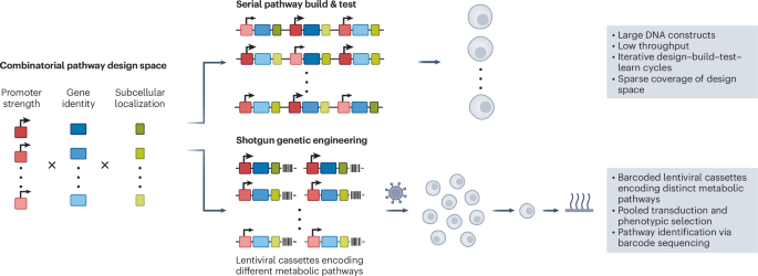
      Article  Google Scholar 

    2. Petzold, C. J., Chan, L. J. G., Nhan, M. & Adams, P. D. Front. Bioeng. Biotechnol. 3, 135 (2015).

      Article  PubMed  PubMed Central  Google Scholar 

    3. Liberante, F. G. & Ellis, T. Curr. Opin. Syst. Biol. 25, 1–10 (2021).

      Article  CAS  Google Scholar 

    4. Rai, K. & O’Connell, R. W. et al. Nature 650, 1035–1044 (2026).

      Article  CAS  PubMed  Google Scholar 

    5. Payne, S. H. & Loomis, W. F. Eukaryot. Cell 5, 272–276 (2006).

      Article  CAS  PubMed  PubMed Central  Google Scholar 

    6. Trolle, J. et al. eLife 11, e72847 (2022).

      Article  CAS  PubMed  PubMed Central  Google Scholar 

    7. Rai, K., Wang, Y., O’Connell, R. W., Patel, A. B. & Bashor, C. J. Curr. Opin. Biomed. Eng. 31, 100553 (2024).

      Article  CAS  Google Scholar 

    8. Zhao, Y. et al. Nat. Biotechnol. 42, 1693–1704 (2024).

      Article  CAS  PubMed  Google Scholar 

    9. Wang, N. B., Beitz, A. M. & Galloway, K. E. Curr. Opin. Syst. Biol. 24, 18–31 (2020).

      Article  PubMed  PubMed Central  Google Scholar 

    10. Brixi, G. et al. Nature 652, 1349–1361 (2026).

      Article  CAS  PubMed  PubMed Central  Google Scholar 

    Download references

    Author information

    Author notes

    1. Kshitij Rai

      Present address: Department of Genome Sciences, University of Washington, Seattle, WA, USA

    Authors and Affiliations

    1. Department of Bioengineering, Rice University, Houston, TX, USA

      Kshitij Rai & Caleb J. Bashor

    2. Graduate Program in Systems, Synthetic and Physical Biology, Rice University, Houston, TX, USA

      Kshitij Rai

    3. Department of Biosciences, Rice University, Houston, TX, USA

      Caleb J. Bashor

    4. Rice Synthetic Biology Institute, Rice University, Houston, TX, USA

      Caleb J. Bashor

    Authors

    1. Kshitij Rai
    2. Caleb J. Bashor

    Corresponding author

    Correspondence to Caleb J. Bashor.

    About this article

    Check for updates. Verify currency and authenticity via CrossMark

    Cite this article

    Rai, K., Bashor, C.J. Shotgun engineering fires up mammalian metabolic design. Nat Biotechnol (2026). https://doi.org/10.1038/s41587-026-03329-4

    Download citation

    • Published:

    • Version of record:

    • DOI: https://doi.org/10.1038/s41587-026-03329-4

  • The “glue” holding your cells together has a surprising second job

    The “glue” holding your cells together has a surprising second job

    A protein best known for helping cells and tissues stay connected has another unexpected role. Researchers have found that it also helps epithelial cells, which form continuous sealed layers throughout the body, engulf nearby dead cells.

    The discovery could have implications for chronic inflammation. Debris from dying cells is a major contributor to inflammatory responses, so understanding how tissues remove that material may reveal new clues about what happens when the cleanup process fails.

    The study, published in Nature Communications, focuses on the E-cadherin complex. This molecular system includes E-cadherin along with three additional proteins. Together, they connect epithelial cells lining areas such as the skin, gut and airways, giving tissues the structural strength they need to remain intact. In these tissues, each cell connects to E-cadherin molecules on neighboring cells.

    Cellular Glue Takes on a Cleanup Role

    A team led by Verena Ruprecht examined epithelial tissues in living zebrafish and mouse embryos. They found that the same molecular machinery also gathers at the exact location where a dying cell comes into contact with the tissue.

    The researchers wanted to know whether E-cadherin and its partners were attaching to the dying cell in the same way they normally attach neighboring epithelial cells. To test that possibility, they carried out two experiments.

    First, they presented the tissue with dying cells that had been stripped of E-cadherin. The epithelial tissue removed those cells just as effectively as it removed normal dying cells. Next, the team introduced fat droplets that contained no protein at all but carried a signal normally displayed on the surface of dying cells. The epithelial cells engulfed those droplets as well.

    “We were intrigued to find out that epithelial cells repurpose their molecular adhesion machinery — the ‘glue’ that normally holds them together — to engulf dying cells,” says ICREA Research Professor Verena Ruprecht, senior author of the study.

    How Cells Eat Without Breaking the Barrier

    Engulfing something roughly the size of another cell presents a difficult mechanical problem. Epithelial cells are tightly packed into barriers that often need to remain sealed, even while individual cells reshape themselves to remove debris.

    Live imaging revealed how they accomplish this. The upper and lower surfaces of the same epithelial cell can behave differently from one another. The lower surface stretches and bends around the dead cell, while the opposite side remains relatively unchanged.

    That upper surface, which may face the outside environment or an open space such as the inside of a lumen, continues maintaining the tissue barrier. Measurements taken before, during and after engulfment showed that the area of the upper surface changed very little. By contrast, the lower surface underwent substantial deformation during the ‘eating’ process.

    Ruprecht compares the behavior to a row of dancers standing with their arms linked. Their upper bodies remain steady while their feet perform increasingly complicated movements when a dying cell appears. “It’s the same dancer with a different choreography,” she says.

    A Molecular Rope and Brake

    The researchers also examined the mechanics that allow the cells to perform this cleanup.

    One protein in the E-cadherin complex acted much like a rope. It connected the molecular assembly to the cell’s internal skeleton, allowing force to be transmitted across the surface of the material being engulfed. When cells lacked this tethering protein, or lacked the specific region that attaches it to the skeleton, they could no longer swallow dead cells.

    Another component behaved more like a brake on the cell’s contractile machinery. Surprisingly, removing this brake did not make the cleanup process more effective. Instead, the cell became too stiff and lost its ability to properly remove dying cells.

    The Same Mechanism Appears in Mammals

    The team next investigated whether the process extends beyond zebrafish.

    In early mouse embryos, blocking E-cadherin caused dying cells to remain uncleared. This matched the results seen in zebrafish and suggests that the mechanism is shared among vertebrates.

    The new work builds on earlier research from Ruprecht showing that embryos can use epithelial tissues to cooperatively remove dying cells. That behavior represents a form of early innate immune defense.

    Embryos are particularly useful for studying these events because they are transparent. Researchers can observe living cells and tissues directly at a level of detail that cannot currently be achieved inside the human body.

    Could the Same Process Work in Adult Tissues?

    An important question remains unanswered. Researchers do not yet know whether this same E-cadherin dependent mechanism operates in adult zebrafish or mice, or in any type of human tissue.

    There are reasons to think it could. Epithelial tissues in adults are already known to remove dying cells in places including the retina, colon, airways and mammary gland. E-cadherin is also found throughout epithelial tissues in the body, and its structure has remained remarkably similar across species. Those characteristics make it a strong candidate for a more broadly used cleanup mechanism.

    The potential medical importance comes from what can happen when dead cells are not removed efficiently. Dying cells that remain in tissues can eventually rupture and release their contents, contributing to chronic inflammation.

    The findings suggest that successful cleanup depends on more than receiving the correct chemical signal to engulf apoptotic debris. Cells must also be physically capable of changing shape, applying force and wrapping around dead material without compromising themselves or the surrounding tissue.

    “Studying the mechanisms of how dying cells can be removed efficiently from tissues is of very high relevance to human health,” concludes Ruprecht.

    The work was led by joint first authors Hanna-Maria Häkkinen, Marta Batet Palau and Laura F. Bianchi and supervised by Verena Ruprecht. It was funded by the Spanish Ministry of Science and Innovation, the Human Frontier Science Program, the European Union’s Horizon Europe program, and the “la Caixa” Foundation, with additional support from the European Social Fund. It made use of the CRG Core Facilities for Advanced Light Microscopy, Tissue Engineering and Protein Technologies.

  • Detectrons convert transient RNA sequences into stable DNA barcodes for high-throughput analysis of RNA-dependent processes

    Detectrons convert transient RNA sequences into stable DNA barcodes for high-throughput analysis of RNA-dependent processes

    Data availability

    Sequencing data associated with this study are available from the National Center for Biotechnology Information Sequence Read Archive under BioProject (PRJNA1366125). Statistical source data underlying the figures are provided in Source Data. Complete variant, plasmid, primer and statistical summary information are provided in Supplementary Tables. Source data are provided with this paper.

    Code availability

    Custom code used to process and analyze data from this study is available through the Shipman Lab GitHub repository (https://github.com/Shipman-Lab/Detectron).

    References

    1. Betzer, O. et al. In vivo neuroimaging of exosomes using gold nanoparticles. ACS Nano 11, 10883–10893 (2017).

      Article  CAS  PubMed  Google Scholar 

    2. Sheth, R. U., Cabral, V., Chen, S. P. & Wang, H. H. Manipulating bacterial communities by in situ microbiome engineering. Trends Genet. 32, 189–200 (2016).

      Article  CAS  PubMed  PubMed Central  Google Scholar 

    3. Ganeshan, S. D. & Hosseinidoust, Z. Phage therapy with a focus on the human microbiota. Antibiotics 8, 131 (2019).

      Article  CAS  Google Scholar 

    4. Zhan, Y., Buchan, A. & Chen, F. Novel N4 bacteriophages prevail in the cold biosphere. Appl. Environ. Microbiol. 81, 5196–5202 (2015).

      Article  CAS  PubMed  PubMed Central  Google Scholar 

    5. Green, A. A., Silver, P. A., Collins, J. J. & Yin, P. Toehold switches: de novo-designed regulators of gene expression. Cell 159, 925–939 (2014).

      Article  CAS  PubMed  PubMed Central  Google Scholar 

    6. Green, A. A. et al. Complex cellular logic computation using ribocomputing devices. Nature 548, 117–121 (2017).

      Article  CAS  PubMed  PubMed Central  Google Scholar 

    7. Pardee, K. et al. Rapid, low-cost detection of Zika virus using programmable biomolecular components. Cell 165, 1255–1266 (2016).

      Article  CAS  PubMed  Google Scholar 

    8. Takahashi, M. K. et al. A low-cost paper-based synthetic biology platform for analyzing gut microbiota and host biomarkers. Nat. Commun. 9, 3347 (2018).

      Article  PubMed  PubMed Central  Google Scholar 

    9. Yan, Z. et al. Programmable fluorescent aptamer-based RNA switches for rapid identification of point mutations. Nat. Chem. 17, 1826–1838 (2025).

      Article  CAS  PubMed  Google Scholar 

    10. Yan, Z. et al. Rapid, multiplexed, and enzyme-free nucleic acid detection using programmable aptamer-based RNA switches. Chem 10, 2220–2244 (2024).

      Article  CAS  PubMed  PubMed Central  Google Scholar 

    11. Zhou, Y. et al. Conditional RNA interference in mammalian cells via RNA transactivation. Nat. Commun. 15, 6855 (2024).

      Article  CAS  PubMed  PubMed Central  Google Scholar 

    12. Millman, A. et al. Bacterial retrons function in anti-phage defense. Cell 183, 1551–1561 (2020).

      Article  CAS  PubMed  Google Scholar 

    13. Yee, T., Furuichi, T., Inouye, S. & Inouye, M. Multicopy single-stranded DNA isolated from Myxococcus xanthus. Cell 38, 203–209 (1984).

      Article  CAS  PubMed  Google Scholar 

    14. González-Delgado, A. et al. Simultaneous multi-site editing of individual genomes using retron arrays. Nat. Chem. Biol. 20, 1482–1492 (2024).

      Article  PubMed  PubMed Central  Google Scholar 

    15. Crawford, K. D., Khan, A. G., Lopez, S. C., Goodarzi, H. & Shipman, S. L. High-throughput variant libraries and machine learning yield design rules for retron gene editors. Nucleic Acids Res. 53, gkae123 (2025).

      Article  Google Scholar 

    16. Khan, A. G. et al. An experimental census of retrons for DNA production and genome editing. Nat. Biotechnol. 43, 914–922 (2024).

      Article  PubMed  PubMed Central  Google Scholar 

    17. Lopez, S. C., Crawford, K. D., Lear, S. K., Bhattarai-Kline, S. & Shipman, S. L. Precise genome editing across kingdoms of life using retron-derived DNA. Nat. Chem. Biol. 18, 199–206 (2022).

      Article  CAS  PubMed  Google Scholar 

    18. Kong, X. et al. Precise genome editing without exogenous donor DNA via retron editing system in human cells. Protein Cell 12, 899–902 (2021).

      Article  CAS  PubMed  PubMed Central  Google Scholar 

    19. Zhao, B., Chen, S. A. A., Lee, J. & Fraser, H. B. Bacterial retrons enable precise gene editing in human cells. CRISPR J. 5, 31–39 (2022).

      Article  CAS  PubMed  PubMed Central  Google Scholar 

    20. Lim, D. & Maas, W. K. Reverse-transcriptase-dependent synthesis of a covalently linked, branched DNA–RNA compound in E. coli B. Cell 56, 891–904 (1989).

      Article  CAS  PubMed  Google Scholar 

    21. Palka, C., Fishman, C. B., Bhattarai-Kline, S., Myers, S. A. & Shipman, S. L. Retron reverse-transcriptase termination and phage defense are dependent on host RNase H1. Nucleic Acids Res. 50, 3490–3504 (2022).

      Article  CAS  PubMed  PubMed Central  Google Scholar 

    22. Chen, T. & Guestrin, C. XGBoost: a scalable tree boosting system. In Proc. 22nd ACM SIGKDD International Conference on Knowledge Discovery and Data Mining (eds Krishnapuram, B. & Shah, M.) 785–794 (ACM, 2016).

    23. Gootenberg, J. S. et al. Nucleic acid detection with CRISPR–Cas13a/C2c2. Science 356, 438–442 (2017).

      Article  CAS  PubMed  PubMed Central  Google Scholar 

    24. Kellner, M. J., Koob, J. G., Gootenberg, J. S., Abudayyeh, O. O. & Zhang, F. SHERLOCK: nucleic acid detection with CRISPR nucleases. Nat. Protoc. 14, 2986–3012 (2019).

      Article  CAS  PubMed  PubMed Central  Google Scholar 

    25. Gootenberg, J. S. et al. Multiplexed and portable nucleic acid detection platform with Cas13, Cas12a, and Csm6. Science 360, 439–444 (2018).

      Article  CAS  PubMed  PubMed Central  Google Scholar 

    26. Jiao, C. et al. Noncanonical crRNAs derived from host transcripts enable multiplexable RNA detection by Cas9. Science 370, 1087–1094 (2020).

      Google Scholar 

    27. McKenna, A. et al. Whole-organism lineage tracing by combinatorial and cumulative genome editing. Science 353, aaf7907 (2016).

      Article  PubMed  PubMed Central  Google Scholar 

    28. Frieda, K. L. et al. Synthetic recording and in situ readout of lineage information in single cells. Nature 541, 107–111 (2017).

      Article  CAS  PubMed  Google Scholar 

    29. Perli, S. D., Cui, C. H. & Lu, T. K. Continuous genetic recording with self-targeting CRISPR–Cas in human cells. Science 353, aag0511 (2016).

      Article  PubMed  Google Scholar 

    30. Choi, J. et al. A time-resolved, multi-symbol molecular recorder via sequential genome editing. Nature 608, 98–107 (2022).

      Article  CAS  PubMed  PubMed Central  Google Scholar 

    31. Tang, W. & Liu, D. R. Rewritable multi-event analog recording in bacterial and mammalian cells. Science 360, eaap9751 (2018).

      Article  Google Scholar 

    32. Farzadfard, F. et al. Single-nucleotide-resolution computing and memory in living cells. Mol. Cell 75, 769–780.e4 (2019).

      Article  CAS  PubMed  PubMed Central  Google Scholar 

    33. Shipman, S. L., Nivala, J., Macklis, J. D. & Church, G. M. Molecular recordings by directed CRISPR spacer acquisition. Science 353, aaf1175 (2016).

      Article  PubMed  PubMed Central  Google Scholar 

    34. Bhattarai-Kline, S. et al. Recording gene expression order in DNA by CRISPR addition of retron barcodes. Nature 608, 217–225 (2022).

      Article  CAS  PubMed  PubMed Central  Google Scholar 

    35. Sheth, R. U., Yim, S. S., Wu, F. L. & Wang, H. H. Multiplex recording of cellular events over time on CRISPR biological tape. Science 374, eabi5919 (2021).

      Google Scholar 

    36. Farzadfard, F. & Lu, T. K. Genomically encoded analog memory with precise in vivo DNA writing in living cell populations. Science 346, 1256272 (2014).

      Article  PubMed  PubMed Central  Google Scholar 

    37. Roquet, N., Soleimany, A. P., Ferris, A. C., Aaronson, S. & Lu, T. K. Synthetic recombinase-based state machines in living cells. Science 353, aad6350 (2016).

      Article  Google Scholar 

    38. Mosberg, J. A., Gregg, C. J., Lajoie, M. J., Wang, H. H. & Church, G. M. Improving lambda red genome engineering in Escherichia coli via rational removal of endogenous nucleases. PLoS ONE 7, e44638 (2012).

      Article  CAS  PubMed  PubMed Central  Google Scholar 

    Download references

    Acknowledgements

    We thank K. S. Pollard for discussions regarding machine learning, K. D. Crawford for discussions regarding Detectron library construction and A. G. Delgado for assistance in assessing Detectron portability.

    Funding

    Work was supported by funding from the Bachrach Family Foundation and the Robert J. Kleberg, Jr. and Helen C. Kleberg Foundation. S.L.S. is a San Francisco Biohub Investigator.

    Author information

    Authors and Affiliations

    1. Gladstone Institute of Data Science and Biotechnology, San Francisco, CA, USA

      Jihoon Han & Seth L. Shipman

    2. Department of Bioengineering and Therapeutic Sciences, University of California, San Francisco, San Francisco, CA, USA

      Seth L. Shipman

    3. Chan Zuckerberg Biohub San Francisco, San Francisco, CA, USA

      Seth L. Shipman

    Authors

    1. Jihoon Han
    2. Seth L. Shipman

    Contributions

    J.H., conceptualization, methodology, investigation, writing, visualization and supervision. S.L.S., conceptualization, methodology, supervision, project administration and funding acquisition.

    Corresponding author

    Correspondence to Seth L. Shipman.

    Ethics declarations

    Competing interests

    J.H. and S.L.S. are named inventors on US provisional patent application no. 63/900,194, related to the technologies described in this work.

    Peer review

    Peer review information

    Nature Biotechnology thanks Alexander Green, Baojun Wang and the other, anonymous, reviewer(s) for their contribution to the peer review of this work. Peer reviewer reports are available.

    Additional information

    Publisher’s note Springer Nature remains neutral with regard to jurisdictional claims in published maps and institutional affiliations.

    Extended data

    Extended Data Fig. 1 Detectrons specifically respond to target RNA expressed under an inducible promoter.

    a, Schematic of the experimental promoters used to express No Toehold control, Detectron, and trigger RNA, along with representations of the expressed transcripts. msr, multicopy single-stranded RNA. msd, multicopy single-stranded DNA. trigRNA, trigger RNA. b, Representative urea PAGE analysis of RT-DNA from the No Toehold control (lane 1, excluding ladder) and from Detectron in the absence (lane 2) or presence of trigger RNA expressed under the pBAD promoter (lane 3), or in the absence (lane 4) or presence of scrambled RNA expressed under the pBAD promoter (lane 5). The experiment was repeated independently three times with similar results.

    Extended Data Fig. 2 Construction of the Detectron variant library.

    a, Schematic of retron Eco1 ncRNA variants tested. b, Representative urea PAGE analysis of RT-DNA from the indicated ncRNA variants (lanes 1-4, excluding ladder) and wild-type (WT) ncRNA (lane 5). c, Representative urea PAGE analysis of RT-DNA from the No Toehold control (lane 1, excluding ladder) and Detectron-V1 in the absence (lane 2) or presence of trigger RNA expressed under the J23105 promoter (lane 3) or J23100 promoter (lane 4). The experiments shown in b and c were repeated independently three times with similar results. d, Design of Detectron variant oligonucleotides. The invariable region containing the full msr and partial msd sequences was omitted from synthesized oligos. e, Pooled oligos were cloned into either on (constitutively expressing trigger RNA) or off (no trigger RNA expression) backbones via SapI digestion. The invariable region was subsequently reinserted into both on and off libraries via BsaI digestion.

    Source data

    Extended Data Fig. 3 Effect of shorter loop lengths on Detectron performance.

    a, Schematic of the focused loop-length analysis. To isolate the effect of loop length from changes in a2 length, a2 was fixed at 12 nt by excluding the loop from the a2 sequence, while loop length was varied from 12 nt to shorter lengths of 11, 9, 7, 5, 3, and 1 nt. b, Enrichment of RT-DNA + plasmid over plasmid alone for Detectrons with the indicated loop lengths, as measured by qPCR; One-way ANOVA followed by two-sided Tukey’s multiple comparisons test with adjustment for multiple comparisons for on-state signal: 11 nt versus 12 nt: P = 0.0970; 9 nt versus 12 nt: P = 0.995; 7 nt versus 12 nt: P = 4.82 × 10⁻⁷; 5 nt versus 12 nt: P = 3.35 × 10⁻¹⁰; 3 nt versus 12 nt: P = 3.35 × 10⁻⁸; 1 nt versus 12 nt: P = 0.543. Closed circles indicate three biological replicates. Bars represent the mean (±s.d.) of three biological replicates. c, on/off ratios of Detectrons with the indicated loop lengths; One-way ANOVA followed by two-sided Tukey’s multiple comparisons test with adjustment for multiple comparisons: 11 nt versus 12 nt: P = 0.230; 9 nt versus 12 nt: P = 0.374; 7 nt versus 12 nt: P = 5.62 × 10⁻⁸; 5 nt versus 12 nt: P = 1.44 × 10⁻¹⁰; 3 nt versus 12 nt: P = 4.13 × 10⁻⁶; 1 nt versus 12 nt: P = 0.430. Bars represent the mean (±s.d.) of three biological replicates.

    Source data

    Extended Data Fig. 4 Machine learning-based model training identifies optimal structural feature set for Detectron performance prediction.

    a, Schematic of the machine learning workflow using XGBoost regression trained on the indicated feature sets. b, Model performance for each fold was evaluated using coefficient of determination (R2), root mean squared error (RMSE), mean absolute error (MAE), and Pearson’s correlation coefficient (r). c, Average of performance metrics across the five outer cross-validation folds. d, Paired t-tests comparing performance metrics between the indicated feature-set models.

    Extended Data Fig. 5 Average on/off ratios and SHAP feature effects across Detectron structural parameters.

    a-b, SHAP analysis of on/off ratios across (a) stem2 and (b) stem1 lengths. Each circle represents an individual Detectron variant. Bars represent the mean SHAP value of the variants. c-f, Average on/off ratios across different feature distributions: (c) combined stem lengths; (d) loop lengths; (e) bulge lengths; and (f) distance from stem to priming G. Closed circles indicate three biological replicates. Bars represent the mean (±s.d.) of three biological replicates. g, Average on/off ratios plotted against free energy of the hairpin (ΔGhairpin). Each circle represents an individual Detectron variant.

    Source data

    Extended Data Fig. 6 Effect of extended trigger-complementary stem pairing on Detectron performance.

    a, Normalized on/off ratios of Detectron variants in which stem2 was present (stem2 ≥ 1 bp) and stem1 length was varied. b, Normalized on/off ratios of Detectron variants in which stem2 was absent (stem2 = 0) and stem1 length was varied, such that the full stem consisted of the trigger-complementary stem1 region. In both panels, bulge, loop and d lengths were held constant at 0 nt, 12 nt and 1 nt, respectively.

    Source data

    Extended Data Fig. 7 Target-site selection affects Detectron-V2 performance within gp23 mRNA.

    a, Schematic of four 33-nt target sites selected within the full-length T4 gp23 mRNA. The 25-nt binding region within each target site represents the sequence expected to mediate initial hybridization with the Detectron-V2 switch RNA. Predicted target-site opening energies (ΔGopen) for the 25-nt binding regions were calculated using RNAplfold; lower ΔGopen values indicate greater predicted local accessibility. b, on/off ratios of Detectron-V2 devices targeting the indicated sites, plotted against the predicted opening energy of the corresponding 25-nt binding region. Closed circles indicate three biological replicates. Bars represent the mean of three biological replicates.

    Source data

    Extended Data Fig. 8 MOI-dependent response of T7-targeting Detectron.

    Barcode enrichment from the T7-targeting Detectron strain following infection with T7 phage at the indicated multiplicities of infection (MOIs). For the MOI titration, the initial bacterial density was kept constant and the amount of T7 phage was varied to achieve the indicated MOIs. Barcode abundance was normalized to the WT barcode and plotted as fold change relative to the no-infection control. Bars represent the mean (±s.d.) of three biological replicates.

    Source data

    Supplementary information

    Supplementary Information (download PDF )

    Supplementary Text, Figs. 1–5 and legend.

    Reporting Summary (download PDF )

    Peer Review file (download PDF )

    Supplementary Tables 1–5 (download XLSX )

    Complete Detectron variant and barcode sequence table, including skpp15 primer assignments, variable switch-region sequences, barcode sequences, msd/a2 sequences, padding sequences and full synthesized oligonucleotide sequences with and without padding. Statistical summary table, including statistical tests, sample sizes, exact P values, test statistics, degrees of freedom, confidence intervals, effect sizes and multiple-comparison adjustments where applicable. Plasmid information table, including plasmid names, descriptions and relevant construct information. Detectron and trigger RNA sequences information table, including sequences for Detectron construct and trigger RNA used in this study. Primer sequence table, including primer names and oligonucleotide sequences used in this study.

    Source data

    About this article

    Check for updates. Verify currency and authenticity via CrossMark

    Cite this article

    Han, J., Shipman, S.L. Detectrons convert transient RNA sequences into stable DNA barcodes for high-throughput analysis of RNA-dependent processes. Nat Biotechnol (2026). https://doi.org/10.1038/s41587-026-03334-7

    Download citation

    • Received:

    • Accepted:

    • Published:

    • Version of record:

    • DOI: https://doi.org/10.1038/s41587-026-03334-7

  • Discovery and engineering of avian R2 retrotransposons for all-RNA-mediated targeted DNA integration in human cells

    Discovery and engineering of avian R2 retrotransposons for all-RNA-mediated targeted DNA integration in human cells

    Data availability

    The sequencing data involved in this research have been submitted to the Genome Sequence Archive for Human, a platform under the Beijing Institute of Genomics, Chinese Academy of Sciences (available at https://ngdc.cncb.ac.cn/gsa-human/). As of the paper’s publication date, the data will be open to the public, and the accession number for retrieval is HRA013312 (ref. 48). Source data are provided with this paper.

    Code Availability

    Analytic code for the sequencing data is publicly available at GitHub at https://github.com/YanpingHu/avian_R2 (ref. 49).

    References

    1. Villiger, L. et al. CRISPR technologies for genome, epigenome and transcriptome editing. Nat. Rev. Mol. Cell Biol. 25, 464–487 https://doi.org/10.1038/s41580-023-00697-6 (2024).

    2. Luo, S., Chen, Q., Chen, Y. & Li, W. Biology and utilization of R2 retrotransposons. RNA Biol. 22, 1–8 https://doi.org/10.1080/15476286.2025.2521890 (2025).

      Article  CAS  PubMed  PubMed Central  Google Scholar 

    3. Eickbush, T. H. & Eickbush, D. G. Integration, regulation, and long-term stability of R2 retrotransposons. Microbiol. Spectr. 3, MDNA3-0011-2014 https://doi.org/10.1128/microbiolspec.MDNA3-0011-2014 (2015).

      Article  CAS  PubMed  PubMed Central  Google Scholar 

    4. Kojima, K. K. & Fujiwara, H. Long-term inheritance of the 28S rDNA-specific retrotransposon R2. Mol. Biol. Evol. 22, 2157–2165 https://doi.org/10.1093/molbev/msi210 (2005).

      Article  CAS  PubMed  Google Scholar 

    5. Chen, Y. et al. All-RNA-mediated targeted gene integration in mammalian cells with rationally engineered R2 retrotransposons. Cell 187, 4674–4689 https://doi.org/10.1016/j.cell.2024.06.020 (2024).

    6. Edmonds, K. K. et al. Structure and biochemistry-guided engineering of an all-RNA system for DNA insertion with R2 retrotransposons. Nat. Commun. 16, 6079 https://doi.org/10.1038/s41467-025-61321-z (2025).

      Article  CAS  PubMed  PubMed Central  Google Scholar 

    7. Zhang, X. et al. Harnessing eukaryotic retroelement proteins for transgene insertion into human safe-harbor loci. Nat. Biotechnol. 43, 42–51 https://doi.org/10.1038/s41587-024-02137-y (2025).

      Article  CAS  PubMed  Google Scholar 

    8. Kojima, K. K., Seto, Y. & Fujiwara, H. The wide distribution and change of target specificity of R2 non-LTR retrotransposons in animals. PLoS ONE 11, e0163496 https://doi.org/10.1371/journal.pone.0163496 (2016).

      Article  CAS  PubMed  PubMed Central  Google Scholar 

    9. Kariko, K., Buckstein, M., Ni, H. & Weissman, D. Suppression of RNA recognition by Toll-like receptors: the impact of nucleoside modification and the evolutionary origin of RNA. Immunity 23, 165–175 https://doi.org/10.1016/j.immuni.2005.06.008 (2005).

      Article  CAS  PubMed  Google Scholar 

    10. Thawani, A. et al. Structures of vertebrate R2 retrotransposon complexes during target-primed reverse transcription and after second-strand nicking. Sci. Adv. 11, eadu5533 https://doi.org/10.1126/sciadv.adu5533 (2025).

      Article  CAS  PubMed  PubMed Central  Google Scholar 

    11. Deng, P. et al. Structural RNA components supervise the sequential DNA cleavage in R2 retrotransposon. Cell 186, 2865–2879 https://doi.org/10.1016/j.cell.2023.05.032 (2023).

    12. Wilkinson, M. E., Frangieh, C. J., Macrae, R. K. & Zhang, F. Structure of the R2 non-LTR retrotransposon initiating target-primed reverse transcription. Science 380, 301–308 https://doi.org/10.1126/science.adg7883 (2023).

      Article  CAS  PubMed  PubMed Central  Google Scholar 

    13. Palm, S. M., Horton, C. A., Zhang, X. & Collins, K. Structure and sequence at an RNA template 5′ end influence insertion of transgenes by an R2 retrotransposon protein. RNA 30, 1227–1245 https://doi.org/10.1261/rna.080031.124 (2024).

      Article  CAS  PubMed  PubMed Central  Google Scholar 

    14. Christensen, S. M., Ye, J. & Eickbush, T. H. RNA from the 5′ end of the R2 retrotransposon controls R2 protein binding to and cleavage of its DNA target site. Proc. Natl Acad. Sci. USA 103, 17602–17607 https://doi.org/10.1073/pnas.0605476103 (2006).

      Article  CAS  PubMed  PubMed Central  Google Scholar 

    15. Eickbush, D. G., Burke, W. D. & Eickbush, T. H. Evolution of the R2 retrotransposon ribozyme and its self-cleavage site. PLoS ONE 8, e66441 https://doi.org/10.1371/journal.pone.0066441 (2013).

      Article  CAS  PubMed  PubMed Central  Google Scholar 

    16. Watase, G. J. & Yamashita, Y. M. RNA polymerase II-mediated rDNA transcription mediates rDNA copy number expansion in Drosophila. PLoS Genet. 20, e1011136 https://doi.org/10.1371/journal.pgen.1011136 (2024).

      Article  CAS  PubMed  PubMed Central  Google Scholar 

    17. Yarnall, M. T. N. et al. Drag-and-drop genome insertion of large sequences without double-strand DNA cleavage using CRISPR-directed integrases. Nat. Biotechnol. 41, 500–512 https://doi.org/10.1038/s41587-022-01527-4 (2023).

    18. Pandey, S. et al. Efficient site-specific integration of large genes in mammalian cells via continuously evolved recombinases and prime editing. Nat. Biomed. Eng. 9, 22–39 https://doi.org/10.1038/s41551-024-01227-1 (2025).

    19. Fell, C. W. et al. Reprogramming site-specific retrotransposon activity to new DNA sites. Nature 642, 1080–1089 https://doi.org/10.1038/s41586-025-08877-4 (2025).

    20. Nelson, J. O., Slicko, A. & Yamashita, Y. M. The retrotransposon R2 maintains Drosophilaribosomal DNA repeats. Proc. Natl Acad. Sci. USA 120, e2221613120 https://doi.org/10.1073/pnas.2221613120 (2023).

      Article  CAS  PubMed  PubMed Central  Google Scholar 

    21. Levesque, S., Cosentino, A., Verma, A., Genovese, P. & Bauer, D. E. Enhancing prime editing in hematopoietic stem and progenitor cells by modulating nucleotide metabolism. Nat. Biotechnol. 43, 534–538 https://doi.org/10.1038/s41587-024-02266-4 (2025).

    22. Liu, P. et al. Increasing intracellular dNTP levels improves prime editing efficiency. Nat. Biotechnol. 43, 539–544 https://doi.org/10.1038/s41587-024-02405-x (2024).

    23. Rabouw, H. H. et al. Middle East respiratory coronavirus accessory protein 4a inhibits PKR-mediated antiviral stress responses. PLoS Pathog. 12, e1005982 https://doi.org/10.1371/journal.ppat.1005982 (2016).

      Article  CAS  PubMed  PubMed Central  Google Scholar 

    24. Warga, E., Anderson, J., Tucker, M., Harris, E. & Elmer, J. Transcriptomic analysis of the innate immune response to in vitro transfection of plasmid DNA. Mol. Ther. Nucleic Acids 31, 43–56 https://doi.org/10.1016/j.omtn.2022.11.025 (2023).

      Article  CAS  PubMed  Google Scholar 

    25. Mohajeri, M. H., Figlewicz, D. A. & Bohn, M. C. Intramuscular grafts of myoblasts genetically modified to secrete glial cell line-derived neurotrophic factor prevent motoneuron loss and disease progression in a mouse model of familial amyotrophic lateral sclerosis. Hum. Gene Ther. 10, 1853–1866 https://doi.org/10.1089/10430349950017536 (1999).

      Article  CAS  PubMed  Google Scholar 

    26. Bohl, D., Naffakh, N. & Heard, J. M. Long-term control of erythropoietin secretion by doxycycline in mice transplanted with engineered primary myoblasts. Nat. Med. 3, 299–305 https://doi.org/10.1038/nm0397-299 (1997).

      Article  CAS  PubMed  Google Scholar 

    27. Jimenez, V. et al. FGF21 gene therapy as treatment for obesity and insulin resistance. EMBO Mol. Med. 10, EMMM201708791 https://doi.org/10.15252/emmm.201708791 (2018).

    28. England, C. G., Ehlerding, E. B. & Cai, W. NanoLuc: a small luciferase is brightening up the field of bioluminescence. Bioconjug. Chem. 27, 1175–1187 https://doi.org/10.1021/acs.bioconjchem.6b00112 (2016).

      Article  CAS  PubMed  PubMed Central  Google Scholar 

    29. Camacho, C. et al. BLAST+: architecture and applications. BMC Bioinformatics 10, 421 https://doi.org/10.1186/1471-2105-10-421 (2009).

      Article  CAS  PubMed  PubMed Central  Google Scholar 

    30. Fu, L., Niu, B., Zhu, Z., Wu, S. & Li, W. CD-HIT: accelerated for clustering the next-generation sequencing data. Bioinformatics 28, 3150–3152 https://doi.org/10.1093/bioinformatics/bts565 (2012).

      Article  CAS  PubMed  PubMed Central  Google Scholar 

    31. Jones, P. et al. InterProScan 5: genome-scale protein function classification. Bioinformatics 30, 1236–1240 https://doi.org/10.1093/bioinformatics/btu031 (2014).

      Article  CAS  PubMed  PubMed Central  Google Scholar 

    32. Katoh, K. & Standley, D. M. MAFFT multiple sequence alignment software version 7: improvements in performance and usability. Mol. Biol. Evol. 30, 772–780 https://doi.org/10.1093/molbev/mst010 (2013).

      Article  CAS  PubMed  PubMed Central  Google Scholar 

    33. Nguyen, L. T., Schmidt, H. A., von Haeseler, A. & Minh, B. Q. IQ-TREE: a fast and effective stochastic algorithm for estimating maximum-likelihood phylogenies. Mol. Biol. Evol. 32, 268–274 https://doi.org/10.1093/molbev/msu300 (2015).

      Article  CAS  PubMed  Google Scholar 

    34. Xie, J. et al. Tree Visualization By One Table (tvBOT): a web application for visualizing, modifying and annotating phylogenetic trees. Nucleic Acids Res. 51, W587–W592 https://doi.org/10.1093/nar/gkad359 (2023).

      Article  CAS  PubMed  PubMed Central  Google Scholar 

    35. Crooks, G. E., Hon, G., Chandonia, J. M. & Brenner, S. E. WebLogo: a sequence logo generator. Genome Res. 14, 1188–1190 https://doi.org/10.1101/gr.849004 (2004).

      Article  CAS  PubMed  PubMed Central  Google Scholar 

    36. Gruber, A. R., Lorenz, R., Bernhart, S. H., Neuböck, R. & Hofacker, I. L. The Vienna RNA Websuite. Nucleic Acids Res. 36, W70–W74 https://doi.org/10.1093/nar/gkn188 (2008).

      Article  CAS  PubMed  Google Scholar 

    37. Bernhart, S. H., Hofacker, I. L., Will, S., Gruber, A. R. & Stadler, P. F. RNAalifold: improved consensus structure prediction for RNA alignments. BMC Bioinformatics 9, 474 https://doi.org/10.1186/1471-2105-9-474 (2008).

    38. Weinberg, Z. & Breaker, R. R. R2R-software to speed the depiction of aesthetic consensus RNA secondary structures. BMC Bioinformatics 12, 3 https://doi.org/10.1186/1471-2105-12-3 (2011).

      Article  CAS  PubMed  PubMed Central  Google Scholar 

    39. Chen, P. J. et al. Enhanced prime editing systems by manipulating cellular determinants of editing outcomes. Cell 184, 5635–5652 https://doi.org/10.1016/j.cell.2021.09.018 (2021).

      Article  CAS  PubMed  PubMed Central  Google Scholar 

    40. Clement, K. et al. CRISPResso2 provides accurate and rapid genome editing sequence analysis. Nat. Biotechnol. 37, 224–226 https://doi.org/10.1038/s41587-019-0032-3 (2019).

      Article  CAS  PubMed  PubMed Central  Google Scholar 

    41. Anzalone, A. V. et al. Programmable deletion, replacement, integration and inversion of large DNA sequences with twin prime editing. Nat. Biotechnol. 40, 731–740 https://doi.org/10.1038/s41587-021-01133-w (2022).

      Article  CAS  PubMed  Google Scholar 

    42. Nurk, S. et al. The complete sequence of a human genome. Science 376, 44–53 https://doi.org/10.1126/science.abj6987 (2022).

      Article  CAS  PubMed  PubMed Central  Google Scholar 

    43. Li, H. & Durbin, R. Fast and accurate long-read alignment with Burrows–Wheeler transform. Bioinformatics 26, 589–595 https://doi.org/10.1093/bioinformatics/btp698 (2010).

      Article  CAS  PubMed  PubMed Central  Google Scholar 

    44. An, J. et al. Enhancement of the viability of T cells electroporated with DNA via osmotic dampening of the DNA-sensing cGAS–STING pathway. Nat. Biomed. Eng. 8, 149–164 https://doi.org/10.1038/s41551-023-01073-7 (2024).

    45. Tang, N. et al. TGF-β inhibition via CRISPR promotes the long-term efficacy of CAR T cells against solid tumors. JCI Insight 5, e133977 https://doi.org/10.1172/jci.insight.133977 (2020).

    46. Kumaki, Y., Oda, M. & Okano, M. QUMA: quantification tool for methylation analysis. Nucleic Acids Res. 36, W170–W175 https://doi.org/10.1093/nar/gkn294 (2008).

      Article  CAS  PubMed  PubMed Central  Google Scholar 

    47. Lin, Y. et al. Tissue-specific mRNA delivery and prime editing with peptide–ionizable lipid nanoparticles. Nat. Mater. 25, 133–145 https://doi.org/10.1038/s41563-025-02320-9 (2026).

      Article  CAS  PubMed  Google Scholar 

    48. Chen., Y. et al. Discovery and engineering of avian R2 retrotransposons for all-RNA-mediated targeted DNA integration in human cells. Genome Sequence Archive for Human https://ngdc.cncb.ac.cn/gsa-human/browse/HRA013312 (National Genomics Data Center, 2026).

    49. Chen., Y. et al. Discovery and engineering of avian R2 retrotransposons for all-RNA-mediated targeted DNA integration in human cells. GitHub https://github.com/YanpingHu/avian_R2 (2026).

    Download references

    Acknowledgements

    We would like to thank J. Sun for guidance on T cell manipulation. We also thank the National Stem Cell Resource Center, Institute of Zoology, Chinese Academy of Sciences, for providing the primary HHFs used in this study.

    Funding

    This work was supported by the Strategic Priority Research Program of the Chinese Academy of Sciences (XDA0510400 and XDC0200000 to W.L. and H.W.; the National Natural Science Foundation of China (32225030 and 82488301 to W.L.; 32501337 to Y.C.; 32425035 and T2521004 to H.W.); the National Key Research and Development Program (2024YFA0917300 to W.L. and N.T.; 2019YFA0110800 to W.L.); the Beijing Natural Science Foundation (Z230011 to W.L.); Initiative Scientific Research Program, Institute of Zoology, Chinese Academy of Sciences (2023IOZ0204, 2024IOZ0202, 2025IOZ03); the Agriculture Science and Technology Major Project (W.L. and H.W.); the Postdoctoral Fellowship Program of China Postdoctoral Science Foundation (GZB20240739 to Y.H.) and the New Cornerstone Science Foundation through the XPLORER PRIZE.

    Author information

    Author notes

    1. These authors contributed equally: Yangcan Chen, Yanping Hu, Shengqiu Luo, Bangwei Mao, Na Tang, Chenxin Wang, Yuze Wang.

    Authors and Affiliations

    1. State Key Laboratory of Organ Regeneration and Reconstruction, Institute of Zoology, Chinese Academy of Sciences, Beijing, China

      Yangcan Chen, Yanping Hu, Shengqiu Luo, Bangwei Mao, Na Tang, Chenxin Wang, Yuze Wang, Hanyu Bai, Xinge Wang, Changxian Peng, Qicheng Chen, Jiahui Xiao, Yu Zou, Peng Wang, Rui Niu, Jin Zhang, Yulong Zhao, Chen Liang, Yunlong Wang, Yiyun Li, Junjie Wang, Ng Shyh-Chang, Tuo Wei, Haoyi Wang, Qi Zhou & Wei Li

    2. University of Chinese Academy of Sciences, Beijing, China

      Yangcan Chen, Shengqiu Luo, Bangwei Mao, Yuze Wang, Hanyu Bai, Changxian Peng, Qicheng Chen, Jiahui Xiao, Yu Zou, Rui Niu, Jin Zhang, Yulong Zhao, Chen Liang, Yunlong Wang, Yiyun Li, Junjie Wang, Ng Shyh-Chang, Tuo Wei, Haoyi Wang, Qi Zhou & Wei Li

    3. Beijing Institute for Stem Cell and Regenerative Medicine, Beijing, China

      Yangcan Chen, Yanping Hu, Na Tang, Chenxin Wang, Xinge Wang, Peng Wang, Ng Shyh-Chang, Tuo Wei, Haoyi Wang, Qi Zhou & Wei Li

    Authors

    1. Yangcan Chen
    2. Yanping Hu
    3. Shengqiu Luo
    4. Bangwei Mao
    5. Na Tang
    6. Chenxin Wang
    7. Yuze Wang
    8. Hanyu Bai
    9. Xinge Wang
    10. Changxian Peng
    11. Qicheng Chen
    12. Jiahui Xiao
    13. Yu Zou
    14. Peng Wang
    15. Rui Niu
    16. Jin Zhang
    17. Yulong Zhao
    18. Chen Liang
    19. Yunlong Wang
    20. Yiyun Li
    21. Junjie Wang
    22. Ng Shyh-Chang
    23. Tuo Wei
    24. Haoyi Wang
    25. Qi Zhou
    26. Wei Li

    Contributions

    W.L., Q.Z. and Y.C. conceived the project and designed the experiments. Y.C., Y.H., S.L., B.M., N.T., C.W., Yuze Wang, H.B., X.W., C.P., Q.C., J.X., Y. Zou, P.W., R.N., J.Z., Y. Zhao, C.L., Yunlong Wang, Y.L. and J.W. performed the experiments. W.L., Q.Z., Y.C., Y.H. and S.L. analyzed the data. W.L., Q.Z., Y.C. and H.W. supervised the research. W.L., Q.Z., Y.C., Y.H., S.L., N.S.-C., T.W. and H.W. wrote the paper, assisted by the other authors.

    Corresponding authors

    Correspondence to Yangcan Chen, Haoyi Wang, Qi Zhou or Wei Li.

    Ethics declarations

    Competing interests

    W.L., Q.Z., Y.C., Y.H., S.L., Q.C., X.W. and B.M. have submitted patent applications related to this paper. The other authors declare no competing interests.

    Peer review

    Peer review information

    Nature Biotechnology thanks Lei Qi, Max Wilkinson and the other, anonymous, reviewer(s) for their contribution to the peer review of this work.

    Additional information

    Publisher’s note Springer Nature remains neutral with regard to jurisdictional claims in published maps and institutional affiliations.

    Extended data

    Extended Data Fig. 1 Workflow for mining new R2 retrotransposons in avian genomes.

    a, Computational pipeline for identifying avian R2 retrotransposons. b, Distribution of newly discovered R2 elements across orders of analyzed avian genomes. c, Left: distribution of downloaded avian genomes across different orders; Right: distribution of avian genomes containing full-length R2 elements across different orders.

    Extended Data Fig. 2 Systematic characterization of Region-1 and Region-2 in the R2Tg protein.

    a, Droplet digital PCR (ddPCR) analysis demonstrates that Region-1 truncation markedly impairs the molecular integration efficiency of R2Tg, and this defect can be rescued by HMGN1 fusion. Cp, copies. Statistical analyses were performed using one-way ANOVA with Dunnett’s multiple comparisons test. b, Effect of Region-1 truncation length on R2-mediated gene integration efficiency in HEK293T cells, coupled with donoropt. c, Identification of substituting domains capable for rescuing Region-1 function in HEK293T cells, coupled with donoropt. NLS1/2, Nuclear Localization Signal 1/217; NBD, nucleosome-binding domain; CHUD, chromatin unfolding domain. Statistical analyses were performed using one-way ANOVA with Dunnett’s multiple comparisons test. d, Trans-expression of Region-1 fails to rescue R2-mediated gene integration efficiency in HEK293T cells, coupled with donoropt. Unpaired, two-tailed Student’s t tests. e, Impact of region-2 truncation on R2-mediated gene integration activity in HEK293T cells, coupled with donoropt. Statistical analyses were performed using one-way ANOVA with Dunnett’s multiple comparisons test. f, Statistical analysis of Region-1 length across 165 avian R2 retrotransposon proteins. g, Statistical analysis of length of distinct subregions (Spacer, NTE-2 and partial NTE-1) in Region-2 across 165 avian R2 retrotransposon proteins. h, Evaluating the activity of R2Tg protein with removed nuclear localization signal or repositioned Flag tag in all-RNA experimental systems in HEK293T cells, coupled with donoropt. Unless otherwise stated, data are presented as mean ± standard deviation (SD) from three biological replicates.

    Extended Data Fig. 3 Investigation of the effects of donor RHA length and polyA length on R2-mediated gene integration efficiency.

    a, Impact of donor RNA with varying right homology arm (RHA) and polyA lengths on integration efficiency in HEK293T cells. US, unrelated vector sequence. b, Impact of donor RNA with 4 nt RHA and various polyA lengths in HEK293T cells. c, Integration efficiency of R2Tgv1.1 with donor RNAs containing different nucleotide components after a 4 bp RHA in HEK293T cells. Unless otherwise stated, data are presented as mean ± standard deviation (SD) from three biological replicates.

    Extended Data Fig. 4 Investigation of the effects of 5’ UTR elements on R2-mediated gene integration efficiency.

    a, Statistical analysis of J1/2 region length across 165 avian R2 5’ ribozymes. b, Predicted secondary structure of the J1/2 region in 165 avian R2 5’ ribozymes, inferred via covariation modeling. c, Statistical analysis of the length of non-ribozyme part in 165 R2 5’ UTRs. d, Predicted secondary structure of the non-ribozyme part in avian R2 5’ UTRs from Aves_c1 to c5, inferred via covariation modeling. e, Integration efficiency of R2Tgv1.1 with donor RNAs harboring modified 5’ UTR sequences in HEK293T cells. Sub1–10 denotes substitution of the first 1–10 nt of the 5’ UTR with heterologous sequences to disrupt the J1/2 secondary structure. Statistical analyses were performed using one-way ANOVA with Dunnett’s multiple comparisons test. f, Length distribution of the buffer region in the avian 3’ UTR. g, Nucleotide composition of the buffer region in the avian 3’ UTR. For all graphs, data are represented as mean ± SD from three biological replicates.

    Extended Data Fig. 5 Systematic comparison of the R2 tool design strategy developed in this study with those of previously reported R2 tools.

    a, Summary of the designs of engineered R2 retrotransposons in this study and two prior studies (Study 17 and Study 26). Mini-donor from study2 was used for comparison. St1, study1; St2, study2. b, Comparison of gene integration activity of R2 variants from different designs, with cross-combination validation of R2 proteins and donor RNAs in HEK293T cells. mRNAs encoding R2Tg shared identical codon usage, translational UTRs and poly(A) tail lengths; donor RNAs were constructed as described in the original reports, including their native promoters, terminators and transgene expression cassette orientations. c, Schematic diagram of donor RNAs with varying lengths. d-e, Comparison of the gene integration capacity of R2 tools from different designs using RNA donors with elongated stuffer sequences (d) or RNA donors carrying gene-T2A-GFP expression cassettes (e) in HEK293T cells. f, Schematic of the RNA donors with dual-fluorescence reporter system (GFP and mCherry) for different R2 tools. g, Gating strategy for flow cytometric analysis of dual fluorescence. h, Assessment of the dual-fluorescence gene integration efficiency of R2 tools from different designs. i, Comparison of the integrity of gene integration products mediated by R2 tools from different designs. Statistical analyses were performed using one-way ANOVA with Tukey’s multiple comparisons test. For all graphs, data are represented as mean ± SD from three biological replicates.

    Extended Data Fig. 6 Investigation of the factors influencing differential activity among R2 tools designs.

    a, Replacement of the 5’ UTR in R2Tg donorvx with that derived from Tribolium castaneum significantly reduced the gene integration activity in HEK293T cells. Unpaired, two-tailed Student’s t test. b, Evaluation of integration efficiency mediated by R2Tgv1.1, where donorvx carried 28-nt, 36-nt, or 100-nt left homology arms (LHA) with or without the 5’ UTR and 5’ Cap-1 in different experimental groups in HEK293T cells. c, Analysis of integration efficiency mediated by R2Tgv1.1 with donors harboring different transgene expression constructs (all-RNA system) in HEK293T cells. Reverse constructs: expression cassette opposite to rDNA transcription direction; Forward constructs: cassette aligned with rDNA transcription direction. 1–9 represent different promoter-polyA terminator combinations. MFI: mean fluorescence intensity of GFP+ cells. d, ddPCR quantification of gene integration copy numbers corresponding to the distinct RNA donor constructs in Panel C. e, Correlation analysis between transgene copy number and fluorescence intensity for all constructs in Panel C via linear regression. Fluorescence intensity of each sample was calculated as MFI multiplied by the percentage of GFP+ cells, reflecting the relative total fluorescence intensity of each sample. f, Correlation analysis between transgene copy number and fluorescence intensity for CMV-containing constructs in Panel C via linear regression. g, Percentage and MFI of GFP+ cells after transfection of corresponding IVT-donor plasmids using Lipofectamine 3000 in HEK293T cells. For all graphs, data are represented as mean ± SD from three biological replicates.

    Extended Data Fig. 7 Systematic characterization of the R2 tools in terms of transgene copy number, integration specificity and full-length insertion capacity in HEK293T cells.

    a, R2 transgene integration copy numbers in the human genome, quantified via ddPCR. Unpaired, two-tailed Student’s t tests. b, Linear regression analysis of total fluorescence intensity versus corresponding transgene copy numbers. Fluorescence intensity of each sample was calculated as MFI multiplied by the percentage of GFP+ cells, reflecting the relative total fluorescence intensity of each sample. c, Whole-genome sequencing showing high on-target integration specificity of R2 retrotransposons in mammalian cells. d, Assessment of the integrity of R2-integrated transgene via whole-genome sequencing. e–j, Investigation of factors influencing the full-length transgene insertion proportion of the R2 retrotransposon tool using the GFP-T2A-mCherry dual-fluorescence reporter system; (e) Percentage of fluorescence-positive cells and (f) proportion of full-length transgene insertions (assessing effects of donor designs). FC, forward construct. Statistical analyses were performed using one-way ANOVA with Dunnett’s multiple comparisons test. (g) Percentage of fluorescence-positive cells and (h) proportion of full-length transgene insertions (assessing effects of R2Tg protein designs). Unpaired, two-tailed Student’s t tests. (i) Percentage of fluorescence-positive cells and (j) proportion of full-length transgene insertions (assessing effects of delivery reagents). Unpaired, two-tailed Student’s t tests. Unless otherwise stated, data are presented as mean ± standard deviation (SD) from three biological replicates.

    Extended Data Fig. 8 Long-term monitoring of transgene expression mediated by R2 integration in HEK293T cells.

    a, Percentage (left) and MFI (right) of GFP+ cells during long-term continuous culture after R2-mediated integration. b, Copy numbers of integrated transgenes during long-term culture (from Extended Data Fig. 8a). Paired, two-tailed Student’s t test. c, Mixed culture of GFP+ cells (from Extended Data Fig. 8a) and negative cells (1:1 ratio) shows faster decline in GFP+ percentage than predicted. Predicted GFP+ percentage: half the positive value from Extended Data Fig. 8a at corresponding days; predicted MFI: MFI of GFP+ cells from Extended Data Fig. 8a. d, CRISPR-Cas9-induced rDNA recombination reduces the percentage and MFI of GFP+ cells; notably, nCas9(H840A)+sg1 did not induce a significant GFP+% and MFI reduction. e–f, Targeted deep sequencing analysis of indel frequencies at rDNA loci induced by the endonuclease activity of R2 retrotransposons (e) or Cas9 (f). Indel frequencies were defined as the proportion of rDNA loci containing indels relative to the total rDNA pool, normalized by subtracting background values from negative controls. g, Sorted GFP+ cells (from Extended Data Fig. 8a) sustain stable and high-efficiency transgene expression during long-term culture. h-i, Transfection of R2 protein-encoding mRNA into stably GFP-expressing cells (derived from Extended Data Fig. 8 g) induced indel formation ( < 0.1%) at rDNA loci (h); however, this did not compromise the percentage of GFP+ cells or MFI (i). END means R2 protein with inactivated active site of RLE domain; RTD means R2 protein with inactivated active site of the RT domain. j–k, Investigation of the effects of different mass ratios of R2 protein-encoding mRNA and donor RNA on transgene expression stability, with the total delivered mass maintained at 1.5 μg. Donor RNA carrying the CMV-GFP transgene (j) and CMV-scFv-T2A-GFP transgene (k) were tested. The R2Tgv1.1 R1119A mutant, derived from the previously described “endoculease-tuned” variants7, was included; residue 1119 corresponds to the amino acid numbering of wild-type R2Tg. All timelines described above are based on Extended Data Fig. 8a. Unless otherwise stated, data are presented as mean ± standard deviation (SD) from three (j–k) or five (a–i) biological replicates.

    Extended Data Fig. 9 Systematic investigation of gene integration mediated by newly mined and engineered R2SPs retrotransposons in primary T cells.

    a, Screening of viral proteins (Vp1 to Vp6) to enhance R2-mediated integration activity in T cells. Paired, two-tailed Student’s t test. b–g, Systematic assessment of the effects of the R2 tool and Vp4 (MERS-CoV-ORF4a) on primary T cell, with relevant parameters quantified at specified time points. (b) Percentage of GFP+ T cells with GFP gene integration at Day 2; (c) MFI of GFP+ T cells with GFP gene integration at Day 2; (d) Viable cell numbers over input at Day 2 post-electroporation; (e) Cell expansion fold-change at Day 10 relative to Day 2; (f) T cell viability rate at Day 2; (g) T cell viability rate at Day 10. END means R2 protein with inactivated active site of the endonuclease domain; RTD means R2 protein with inactivated active site of the RT domain; Q9P means Vp4 protein with inactivated active site of the RNA-binding domain23. h–i, Whole-genome sequencing demonstrating that Vp4 exerts minimal effects on R2 retrotransposons integration specificity (h) and full-length insertion (g) in human primary T cells. Data were obtained using Day 2 samples (from Extended Data Fig. 9b). j, ddPCR quantification of transgene copy numbers in T cells treated by different components (data collected at Day 2). k, long-term monitoring of transgene copy number changes in T cells via ddPCR. l, Integration of longer RNA donors (CMV-scFv-T2A-GFP) in primary T cells using the R2SPsv1.2 tool; long-term detection of GFP+ cell percentage and MFI. m, long-term monitoring of transgene copy number changes in T cells with integrated longer transgene (corresponding to Extended Data Fig. 9 l) via ddPCR. n, Assessment of DNA methylation dynamics at the CMV promoter of integrated transgenes in Day 2 and Day 12 samples (from Extended Data Fig. 9 l) via bisulfite sequencing. o, Investigation of the effects of transgene constructs with distinct promoters or transgene-expressing orientation on transgene expression stability in primary T cells. p, Palbociclib treatment attenuates the decline in GFP+% and GFP signal intensity. q, Palbociclib treatment reduces the proliferation rate of primary T cells. r–s, Integration of the CAR-CD19 transgene in primary T cells using the engineered R2SPsv1.2 tool. (r) Percentage of CAR-CD19-positive cells at Day 2; (s) Percentage of CAR-CD19-positive cells at Day 10. t, Cytotoxicity assay of R2-edited CAR-T cells via coculture with target tumor cells. Unless otherwise stated, data are presented as mean SD from 3 biological replicates from different T cell donors.

    Extended Data Fig. 10 Systematic investigation of gene integration mediated by newly mined and engineered R2SPs retrotransposons in human primary NK cells.

    a–f, Systematic assessment of the effects of the R2 tool and Vp4 on human primary NK cell status, with relevant parameters quantified at specified time points. (a) Dynamic changes in GFP+ cell percentage and MFI of NK cells with GFP gene integration from Day 2 to Day 6 (a subset of R2-treated NK cells was reactivated at Day 2); (b) Monitoring transgene copy numbers in NK cells via ddPCR; (c) Viable cell numbers at Day 2 post-electroporation; (d) Cell expansion fold-change at Day 6 relative to Day 2; (e) NK cell viability rate at Day 2; (f) NK cell viability rate at Day 6; n = 3 biological replicates from different NK cell donors. g, Integration of RNA donor harboring CMV-GFP transgene in primary human foreskin fibroblasts using the R2SPsv1.2 tool; long-term detection of GFP+ cell percentage and MFI. n = 3 biological replicates. h, Monitoring transgene copy numbers in HFFs via ddPCR. Unless otherwise stated, data are presented as mean ± SD.

    Supplementary information

    Source data

    About this article

    Check for updates. Verify currency and authenticity via CrossMark

    Cite this article

    Chen, Y., Hu, Y., Luo, S. et al. Discovery and engineering of avian R2 retrotransposons for all-RNA-mediated targeted DNA integration in human cells. Nat Biotechnol (2026). https://doi.org/10.1038/s41587-026-03315-w

    Download citation

    • Received:

    • Accepted:

    • Published:

    • Version of record:

    • DOI: https://doi.org/10.1038/s41587-026-03315-w

  • Behind (cell) walls

    While mammalian delivery technologies are advancing to translation at an exceptional rate, delivery to plant tissues faces challenges, limiting their practical applications.

    Crops genetically engineered for higher environmental stress and herbicide tolerance, enriched nutrition, disease resistance, and carbon sequestration for carbon management are important to meet global food demand. Gene editing technologies appear to promise faster and easier adaptation than traditional breeding approaches. However, to generate a desired genetic edit that is also transmitted across generations, the gene-editing machinery must be delivered to the appropriate plant tissue. In mammals, delivery systems have become increasingly sophisticated, with ongoing improvements in immunogenicity, targeting precision and efficiency1. Plants, however, have distinct physical barriers, have different transport systems (xylem and phloem) and are under continuous environmental stress. Mammalian delivery systems such as lipid nanoparticles (LNPs) are optimized for tissue-specific barriers2 and cannot traverse the plant cell wall. In addition, gene editing of human tissues is restricted to somatic cells to minimize safety concerns. In plants, the opposite is desired: for heritability, delivery systems must be capable of reaching reproductive tissues, or the editing reagents must be applied directly to these cells.

    Growing plants for transformation takes time. The most common method is Agrobacterium-mediated transformation, whereby a natural pathogen transfers DNA containing an editing construct into a mass of undifferentiated plant cells called a callus. The callus can be screened for cells that have successfully been edited, and these cells can regenerate into a whole plant in appropriate culture conditions. Occasionally, other tissues such as the growing meristem or immature embryos can be transformed instead of a callus. As an alternative to Agrobacterium-mediated transformation, DNA has been attached to tiny gold particles that are physically propelled into plant cells through the cell wall and membrane, but DNA integrations using this method can be random, and many cells are damaged or die during the process3. Other approaches, such as viral delivery or regeneration of edited protoplasts that lack cell walls, rely heavily on tissue culture-based or transgenic intermediates, which are often time-consuming, labor-intensive, dependent on genotype and species, and bottlenecked by difficulties in plant regeneration or viral host range4.

    The vast species variety of plants is another limitation. As in mammalian tissue delivery, what works well in one plant may not work in another. For plants, germline or meristematic tissues must be targeted, ideally in a species-agnostic way. Also, as in mammalian cells, edits need to be done efficiently, fast, and at scale.

    Recent cell culture- and transgene-free “in planta” approaches avoid the time-consuming step of tissue culture for regeneration and have produced widespread interest in accelerating heritable editing. In these methods, developmental regulators are co-delivered with gene-editing reagents to induce new shoot meristems and enable heritable genome editing in whole plants5. Another recently published method grafts transgenic rootstocks to wild-type shoots to generate transgene-free offspring in one step6. While applications to tobacco, tomato, potato and grape (and in 2025 to soybean) have been successful, this crop-engineering workflow is not yet routine5.

    Another recent in planta approach, virus-induced genome editing (VIGE), uses viral vectors to transiently deliver gene editing CRISPR components into plant cells directly, with high editing efficiencies and without the need for tissue culture intermediates7,8,9. Common viruses used for VIGE will not work for all plants, and currently the technology is not scalable. Whereas expanding the host range of mammalian viruses often requires altering cell entry viral receptor binding (tropism), broadening the host range of plant viruses may instead depend on overcoming constraints related to replication, systemic spread and host–virus molecular compatibility. VIGE approaches have worked well in dicot species, but their application in major monocot crops such as rice and wheat remains more challenging as a result of a more limited viral vector toolkit8. In addition, the virus must access the plant germline and deliver its payload to the meristem. It will be difficult to find a broadly applicable virus that can act on a wide variety of crops and cultured plants. Adding RNA mobility sequences can help to move the cargo, but not the virus10. Impairing plant immunity gives viruses better access to plant cells, and thus higher delivery efficiencies11, but plant-specific mechanistic and physical barriers are not easy to overcome.

    Working with viruses as delivery technologies in plants also creates regulatory challenges. The use of infectious agents in the food supply requires rigorous demonstration that engineered viruses do not acquire unintended properties, harm non-target species or create new ecological risks. Addressing these regulatory concerns will be essential for broader adoption of such approaches. As an alternative, existing viral vectors with known safety risks could be engineered, with recognized engineering principles potentially adapted to broaden host tropism in plants.

    Lipid nanoparticles (LNPs) have transformed the field of therapeutic genome editing in humans, but their application in plants remains far less developed. LNPs and virus-like particles are already known to carry larger editing machineries in mammalian cells, like those required for prime and base editing, and could be functionalized in plants. LNPs would need to navigate several barriers, including transport to the target tissue, passage through the cell wall, cellular uptake and intracellular cargo release. Nanosheets functionalized with lysozymes have been used to loosen the cell wall in target plants and deliver RNA cargo and plasmid DNA, demonstrating delivery to reproductive tissues (pollen) in tomato. Yet this was limited to GFP nucleic acid delivery; no editing machinery was delivered to enable heritable genome editing12.

    Plant biotechnology companies seem to be striking a balance between investing in advanced transgene- and cell culture-free methods and more traditional routes of transformation. Terrana Biosciences is introducing engineered self-replicating, native plant RNAs into the plant that could move throughout the plant and deliver information or desired traits, avoiding the regeneration bottleneck of traditional methods. Synthetic latent RNAs can travel through the seed of corn, bell peppers and almond. Qi Biodesign is also looking at RNA-based grafting methods and alternative approaches including direct and transient protein delivery to the meristem in plants such as tomato. Vireo modifies plants directly in the greenhouse using shoot generation, also eliminating the need for tissue culture while still editing cells that can produce new shoots. Yet these technologies each need to be optimized with individual adaptions for every species and are not general solutions.

    Considering the magnitude of the challenge and the benefits that time-saving advances could bring, the level of activity in plant delivery systems compared to that in mammalian ones appears modest. Of course, plant transformation approaches that perform efficiently in laboratory genotypes often show substantially reduced efficiency, or may fail altogether, when applied to elite commercial cultivars because of strong genotype dependence in transformation and regeneration processes. This could limit their wider adoption. But this is true for mammalian gene editing technology as well. Today, regulatory requirements for transgene-free approaches in plants vary between countries and are continually being modified to keep up with the pace of advances.

    Gene editing in plants seems no longer primarily limited by the editing machinery itself, but by the ability to deliver it. If the field continues to improve the editor while leaving delivery largely unchanged, the practical reach of gene editing will remain limited by the biology of transformation. But if delivery becomes an equally deliberate target of innovation, the set of plants that can be engineered — and the traits that can be addressed — could expand dramatically.

  • Deep learning perturbation models can outperform baselines on calibrated metrics

    Deep learning perturbation models can outperform baselines on calibrated metrics

    Main

    Genetic perturbation modeling aims to predict the transcriptomic impact of inhibiting or activating one or more genes, with the potential to enable scalable in silico screens for therapeutic target discovery. Recent studies have questioned whether transcriptome-level perturbation modeling is viable. Ahlmann-Eltze et al. reported that deep learning models do not outperform uninformative baselines across multiple datasets1. Likewise, several independent benchmarks have found that a simple ‘mean baseline’, the average perturbed gene expression profile in the training set, often matches or surpasses state-of-the-art models on metrics such as mean absolute error (MAE), mean squared error (MSE) or the correlation of control-referenced deltas (Pearson(Δctrl))2,3,4,5,6,7.

    In earlier work, we identified two artifacts that explain why the mean baseline can appear predictive despite lacking a perturbation-specific signal8. The first, control bias, arises when systematic differences between control and perturbed cells inflate control-referenced correlation metrics, a phenomenon also recently described by Viñas Torné et al.2. The second, signal dilution, occurs when error metrics dilute meaningful biological signals arising from perturbations with a small but significant number of differentially expressed genes (DEGs), causing mean predictions to appear accurate. Together, these effects allow uninformative predictors to achieve deceptively high scores even when they fail to capture underlying biology, highlighting the need to evaluate whether common benchmarking metrics can distinguish uninformative from meaningful predictions in the first place. In experimental biology, positive and negative controls provide a direct means to test this. However, while the mean baseline serves as an intuitive negative control, existing benchmarks typically lack a corresponding positive control, leaving ambiguity when models perform poorly; low scores may reflect either genuine model failure or insufficient metric sensitivity.

    Previously, we proposed the technical-duplicate baseline as a positive control, in which one half of the cells from each perturbation are used to predict the other8 (Fig. 1a). Because both halves share the same perturbation-specific signal, this baseline was expected to outperform uninformative predictors such as the mean baseline. However, when we measured the performance of these baselines on the Norman19 and Replogle22 K562 genome-wide Perturb-seq (GWPS) datasets using MSE and Pearson(Δctrl), we observed mixed results. As expected, the technical duplicate outperformed the mean baseline in Norman19 (Extended Data Fig. 1a,c). In Replogle22 K562 GWPS, however, it performed comparably under Pearson(Δctrl) (Extended Data Fig. 1d) and underperformed on MSE (Extended Data Fig. 1b), both on average and in approximately 95% of perturbations individually (Extended Data Fig. 1e). In our subsequent analysis (detailed in Supplementary Note 1), we traced this discrepancy back to signal dilution; for Replogle22 K562 GWPS, there were only 3.25 DEGs per perturbation on average (versus 102.09 for Norman19) (Supplementary Table 1). Because the mean baseline is a better estimate of unperturbed gene expression versus the technical duplicate (largely because of greater statistical power), it displays more robust performance in datasets that have weaker perturbations on average.

    Fig. 1: Evaluating the calibration of benchmarking metrics.

    a, The technical-duplicate baseline is generated by splitting cells from each perturbation into two groups, using one half to predict the other. b, The interpolated duplicate baseline, which blends the technical-duplicate and mean baseline using a weight α = 1 − PDEGs from DEG analysis (adjusted P value). The more significantly perturbed a gene is, the more interpolation is weighted toward the technical duplicate, while less significant or unperturbed genes are weighted toward the mean baseline. c, DRF measures calibration as the ratio of the empirical gap between positive and negative controls (‘real response’) and the gap between negative controls and perfect metric performance (‘ideal response’). Higher DRF indicates greater metric sensitivity to perturbation-specific signal. d, Box plots of DRF values across perturbations for MSE versus WMSE across all 14 datasets. μΔ is the mean perturbation-wise difference; P is the adjusted P value from paired two-sided Wilcoxon rank-sum tests. Box plots show the median (center line), 25th and 75th percentiles (box bounds) and whiskers extending to the most extreme data points within 1.5× the interquartile range from the box. The number of points within each box is the number of perturbations per dataset (Supplementary Table 1). e, Heat map of mean DRF for 12 benchmarking metrics across all 14 datasets. Bar plots show the mean DRF per dataset (top) and mean DEGs per perturbation (right). Sample size is equal to the number of perturbations per dataset (Supplementary Table 1).

    Motivated by this observation, we introduce an interpolated duplicate baseline that combines the strengths of both approaches by predicting a value between the mean baseline and the technical duplicate, using an interpolation parameter α derived from the DEG P value for each gene (Fig. 1b and Extended Data Fig. 2). Predictions for strongly affected genes are dominated by the technical duplicate, whereas predictions for weakly affected genes are dominated by the mean baseline, yielding consistently positive performance (Extended Data Fig. 3).

    With our positive control (interpolated duplicate) and negative control (mean baseline) in hand, we next defined a meta metric to quantify the calibration of benchmarking metrics. We term this quantity the ‘dynamic range fraction’ (DRF), which measures, for each perturbation, how effectively a metric distinguishes positive from negative controls. For any metric m(⋅), DRF is defined as

    $$,text{DRF},=frac{m({hat{y}}_{p})-m({hat{y}}_{n})}{m(y)-m({hat{y}}_{n})+epsilon }$$

    (1)

    where ({hat{y}}_{n}) is the mean baseline (or any other negative control), ({hat{y}}_{p}) is the interpolated duplicate (or any other positive control), y represents the ground truth and, hence, yields perfect performance on the metric (for example, MSE = 0 or Pearson(Δctrl) = 1) and ϵ is a small constant added for numerical stability. DRF captures the fraction of the theoretical dynamic range ([m(y)-m({hat{y}}_{n})]) (‘ideal response’) that is realized by the empirical range ([m({hat{y}}_{p})-m({hat{y}}_{n})]) (‘real response’) (Fig. 1c). When the positive control outperforms the negative control (and, hence, the metric is better calibrated), DRF values increase in proportion. In a miscalibrated scenario, DRF values approach zero, reflecting limited metric sensitivity to detect improvements over the negative control.

    We applied DRF to assess the calibration of MSE and Pearson(Δctrl) in the Replogle22 K562 GWPS and essential gene datasets9. In both datasets, most perturbations show low DRF values for these metrics (Extended Data Fig. 4a). Consistent with this, SP2 transcription factor (TF) inhibition in Replogle22 K562 GWPS has DRF(MSE) near zero (Extended Data Fig. 4b), yet gene set enrichment analysis (GSEA) of DEG ranks induced by SP2 perturbation recovers SP2 binding targets among the top ENCODE/ChEA gene sets (Extended Data Fig. 4c). A similar pattern was observed across multiple other TFs (that is, DRF(MSE)) near zero despite the presence of meaningful biological signal; Extended Data Fig. 4d and Supplementary Note 1, supporting the notion of signal dilution as a failure mode of MSE.

    If signal dilution drives poor calibration, metrics that emphasize perturbation-specific effects should recover higher DRF. We previously proposed weighted MSE (WMSE)8 for exactly this purpose; WMSE upweights errors on genes with stronger perturbation effects, even when they comprise a small fraction of the transcriptome and, when used as a training objective, WMSE can increase perturbation model output variance and improve performance relative to standard MSE. As expected, WMSE displayed improved calibration relative to MSE, both for individual TF perturbations (Extended Data Fig. 4b) and at the dataset level, even in datasets with few DEGs per perturbation (Fig. 1d and Extended Data Fig. 4E).

    Extending this analysis to 18 metrics spanning complementary objective families—direct reconstruction error, reference-based delta metrics and retrieval-based metrics—we found that widely used metrics such as MSE and Pearson(Δctrl) are often poorly calibrated, unless evaluated in datasets with stronger perturbation strength overall, such as Norman19 (Fig. 1e). In contrast, weighted and rank-based metrics—including WMSE, weighted ({R}_{Delta }^{2}) (same weights as WMSE8) and normalized inverse rank (NIR)—consistently exhibited higher calibration across datasets, reflecting their shared design principle of emphasizing perturbation-specific signal. Likewise, filtering for the top 100 DEGs per perturbation also increased metric calibration in general (Extended Data Fig. 5).

    To evaluate the reliability of our calibration approach, we analyzed the impact of changing the positive and negative controls for DRF calculation, the number of cells per perturbation, sequencing depth per cell or the number of highly variable genes (HVGs) selected and evaluating the relationship between perturbation strength and baseline performance (Supplementary Note 2). Compared to typical benchmarking metrics such as MSE and Pearson Δctrl, we found that well-calibrated metrics (for example, WMSE, weighted ({R}_{Delta }^{2}) and NIR) amplify perturbation-specific signal and maintain higher calibration, even when data quality is lower (that is, lower library size or cell count), perturbations are weaker or selected genes have lower variance on average. Taken together, our analysis reinforces the validity of our calibration framework and utility of the well-calibrated metrics identified here.

    We then used our well-calibrated metrics to measure model performance on the unseen genetic perturbation prediction task, in which models predict responses to individual perturbations held out during training (Fig. 2a, left). Nine models were evaluated: scGPT10, GEARS11, PRESAGE12, scLambda13, CellFlow14 and four foundation model embedding probes (fMLPs) using Geneformer15, ESM2 (ref. 16), scGPT and GenePT17 embeddings. Models span multiple generations of perturbation modeling—helping disentangle the contributions of metric calibration and model development—and we used an MLP probe to evaluate the relative utility of various foundation model embeddings for providing useful perturbation representations. Baselines include the mean baseline, control baseline (average of control cells) and a linear baseline introduced previously1 that involves performing principal component analysis (PCA) on the training set gene expression matrix and fitting a linear model to predict unseen genetic perturbation responses using these features.

    Fig. 2: Benchmarking under well-calibrated metrics for unseen genetic perturbation prediction and unseen combination prediction.

    a, Task overview. In the unseen perturbation task, models train on single perturbations and generalize to held-out ones (Replogle22 K562 and Nadig25 HepG2 datasets). In the unseen combo task, models see all single perturbations plus some combinations during training and then predict held-out gene combos (Wessels23 and Norman19 datasets). b, Forest plot of per-perturbation performance deltas relative to the mean baseline for WMSE in Replogle22 K562, with 95% confidence intervals (n = 2,045). Statistics from paired two-sided t-tests (model versus mean baseline) with Bonferroni correction. c, As in b, but using weighted ({R}_{Delta {rm{ctrl}}}^{2}), where higher is better. d, As in b, but using Pearson(Δpert), where higher is better. e–g, As in b–d, respectively, but for the Wessels23 unseen combo dataset (n = 187).

    In Replogle22 K562, earlier models (scGPT and GEARS) do not outperform baselines under poorly calibrated metrics such as MSE and Pearson(Δctrl) (Extended Data Fig. 6a,b), consistent with prior benchmarks1,2,4,5,7. Under well-calibrated metrics, however, even these earlier models mostly outperform uninformative baselines (Fig. 2b–d and Extended Data Fig. 6c), suggesting that their perturbation-specific signal was present but obscured by metric choice. More recent models (PRESAGE and scLambda) go further, often outperforming uninformative baselines even under poorly calibrated metrics; indeed, on every metric, at least one deep learning model outperforms all baselines (Supplementary Table 2). These findings were also replicated in the independent Nadig25 HepG2 dataset18 (Extended Data Fig. 7 and Supplementary Table 2).

    Using our fMLP probe, we also observed consistent differences in performance between perturbation embedding features, with GenePT and ESM2-based fMLP models proving more predictive overall. These results were found to be consistent across a size ablation study in which we reduced fMLP model capacity to approximately one half and one quarter of the original parameter count and trained in the Replogle22 K562 (Extended Data Fig. 7).

    We next evaluated model performance on the unseen combination prediction task, in which models must predict the transcriptomic response to pairs of perturbed genes after training on each single genetic perturbation and 25% of all combos (Fig. 2a, right).

    We first benchmarked on Norman19, the most widely used dataset for this task1,2,3,4,5,7,19, which comprises 100 single and 124 combo (two-gene) perturbations. The additive baseline (predicts combination effects by summing single effects) performed strongly here, as expected, given that approximately 96% of effects were additive1 and the training set covered only 31 of 4,950 possible pairs (0.63%) (these 31 pairs represent half of the total 62 combinations in our train–validation split; in contrast, the previous study1 used all 62 combinations for training as their benchmark did not include a validation set), leaving little opportunity to learn nonadditive interactions. Most models exceeded mean and control baselines across metrics but the additive baseline remained difficult to surpass (although deep learning models outperformed it on six of 18 metrics). Further analysis shows that the additive baseline captured ~88% of the ideal performance gap in the best-calibrated metrics (Extended Data Fig. 8), comparable to the interpolated duplicate, which has access to held-out combination data. This evidence of additive baseline saturation, together with limited combinatorial coverage, suggests a limit to Norman19’s value for benchmarking models that aim to learn nonadditive genetic interactions and we recommend that future studies refrain from using this dataset as the sole benchmark of combinatorial perturbation modeling.

    To test whether models can surpass additivity when exposed to a greater proportion of the combinatorial landscape during training, we evaluated Wessels23 (ref. 20), which includes 28 single genetic perturbations and 157 unique perturbation pairs (training set covers 10.3% of possible combinations versus 0.63% in Norman19). In this setting, multiple models outperformed the additive baseline under WMSE and weighted ({R}_{Delta {rm{ctrl}}}^{2}) (Fig. 2e,f), and PRESAGE exceeded it on 15 of 18 metrics (Supplementary Table 2), including Pearson(Δctrl) (Fig. 2g). Notably, PRESAGE is a more recent architecture that was developed after the benchmarking studies that established the additive baseline as a robust predictor compared to other models, exemplifying improving trends in model performance over time in this task. Together, these findings demonstrate that deep learning models can outperform the additive baseline when combinatorial coverage is sufficient.

    Our benchmarking revealed that model performance varies substantially across datasets, reflecting differences in task difficulty. Replogle22 K562 and Nadig25 HepG2 pose a challenging unseen genetic perturbation task with weaker perturbations on average (median number of DEGs: one for Replogle22 K562 and zero for Nadig25 HepG2), whereas Wessels23 involves an unseen combination task with stronger perturbations (median number of DEGs: eight) (Supplementary Table 1). Consistent with this, positive control baselines achieve higher scores on Wessels23 than on Replogle22 K562 across all comparable metrics (Supplementary Table 2) and most models show the same pattern, indicating that performance differences across datasets largely track task difficulty rather than model-specific failure modes.

    Our results also show that models exhibit substantial variation across metric families and we caution against treating any single well-calibrated metric as definitive (as discussed for complementary metric families below). For example, scGPT achieves the lowest WMSE among all models in Replogle22 K562 (0.027 ± 0.001) and highest Pearson(Δctrl) on DEGs (0.367 ± 0.009) yet performs poorly on Pearson(Δpert) across all genes (0.081 ± 0.003) (Supplementary Table 2), barely above the mean baseline.

    We also evaluated whether model performance corresponds to recovery of biological insights through an analysis of two downstream tasks: (1) pathway recovery—correlation between GSEA calculated on predicted and ground-truth perturbation effects, which is relevant to pathway analysis from model predictions, and (2) neighborhood-structure recovery—rank-based similarity between KNN graphs constructed from predicted and observed perturbation shifts, which is relevant to perturbation network analysis. Across datasets, models performing strongly under well-calibrated metrics also showed better pathway recovery (Extended Data Fig. 9a–d), with pathway recovery rankings and well-calibrated metric rankings being correlated (Replogle22 K562 ρavg = 0.76; Wessels23 ρavg = 0.84). Neighborhood recovery showed a similar but more variable pattern (Replogle22 K562 ρavg = 0.77; Wessels23 ρavg = 0.58), with the strongest correspondence between neighborhood-structure recovery and retrieval-based NIR/PDS metrics (ρ > 0.78 in all cases), consistent with their related objectives (Extended Data Fig. 9e–h). These results indicate that well-calibrated metrics capture biologically meaningful differences between models relevant to downstream analysis objectives.

    In summary, we found that models frequently outperform uninformative baselines under well-calibrated metrics. This includes earlier models such as scGPT and GEARS, whose perturbation-specific signal was present but obscured by metric choice (Extended Data Fig. 6), and newer models spanning diverse architectures—including PRESAGE (attention-based, prior knowledge embeddings), scLambda (variational autoencoder) and CellFlow (flow matching)—which stand out for their stronger performance relative to uninformative baselines in these metrics. Earlier benchmarking studies had a constructive role in surfacing modeling limitations that these and other architectural advances have begun to address. In our results, PRESAGE is notable both for its strong performance and sophisticated perturbation representation approach based on biological prior knowledge. Concurrently, an independent preprint by Cole et al. systematically benchmarked foundation model and prior-knowledge-based embeddings for perturbation response prediction21. Their work reached complementary conclusions, showing that embeddings encoding prior knowledge can improve prediction, further underscoring the value of prior knowledge for building informative representations of genetic perturbations.

    The DRF calibration framework we introduce here is not tied to a prescriptive definition of positive or negative controls; instead, it provides a general approach for assessing metric sensitivity relative to any reasonably defined performance baselines. Moreover, this framework does not eliminate the need for complementary benchmarking metrics; direct error, reference-based, weighted and retrieval-based metrics each capture distinct aspects of model behavior and should be combined in holistic model evaluations. For instance, direct error metrics are a useful guardrail against rewarding implausible model predictions, as recently demonstrated in the Virtual Cell Challenge22. That being said, we recommend MSE as it showed better calibration overall compared to MAE (Fig. 1e and Extended Data Fig. 5). In practice, a model performing substantially below baselines on either metric would warrant scrutiny regardless of calibration as this may indicate a lack of modeling realism.

    Several limitations remain for this work. First, we focused on the unseen genetic perturbation and unseen combination prediction tasks, leaving the unseen context task (predicting responses in unobserved cell types, donors or conditions) unaddressed. Additionally, the contrast between Norman19 (0.63% of the combinatorial search space in training) and Wessels23 (10.3%) suggests that training set characteristics may influence the performance of both baselines and models; evaluating additional combinatorial datasets will help to characterize this relationship more thoroughly. Lastly, as the field continues to evolve rapidly, conclusions drawn from any fixed set of models necessarily reflect a snapshot of perturbation response modeling and available perturbation datasets at a particular time. Benchmarks should incorporate both earlier and up-to-date architectures to track whether advances in modeling translate to increased performance in well-calibrated benchmarks.

    Overall, our findings reframe the debate on the feasibility of genetic perturbation modeling. A key obstacle has been the reliance upon uncalibrated benchmarks that obscure true model performance. With calibration-aware evaluation, we show that models can outperform uninformative baselines, contextualizing prior reports of model underperformance and helping to establish a more optimistic foundation for genetic perturbation modeling.

    Methods

    Baseline definition

    To evaluate metric calibration and model performance, we define both uninformative and trivial baselines, along with idealized positive control baselines.

    Control baseline

    Computed at the dataset level, the control baseline μc is the averaged expression profile of 8,192 random unperturbed control cells.

    Mean baseline

    Computed at dataset level, it is defined as the average of averages of all train perturbations. Mathematically, given a set of M train perturbations each represented by a set of cells ({mathcal {S}}_{1},{mathcal{S}}_{2},ldots ,{mathcal {S}}_{M}) that can vary in size, the mean baseline is computed as follows:

    $${mu}_{mathrm{all}}=frac{1}{M}mathop{sum}limits_{i=1}^{M}left(frac{1}{| {mathcal{S}}_{i}| }mathop{sum}limits_{jin {mathcal{S}}_{i}}{x}_{i,j}right)$$

    (2)

    where xi,j represents the expression profile of the jth a cell of the ith perturbation. Note that this computation is dense and weights every perturbation equally instead of every cell equally.

    Technical duplicate

    The technical-duplicate baseline is defined by randomly dividing the cell set ({{mathcal{S}}}_{i}) associated with perturbation pi in two: a ground-truth set ({mathcal {S}}_{i,mathrm{GT}}) and a technical-duplicate set ({mathcal {S}}_{i,mathrm{TD}}). The average profiles of both sets μi,GT and μi,TD are then considered the ground-truth and technical-duplicate values for evaluation, respectively. This definition aims to provide an idealized estimate of good performance where the prediction errors are only because of the inherent variability of the experiment. In other words, it answers the following question: If we were to sequence additional cells from the same perturbed biological samples (as in a technical replicate), how predictive would those new cells be of the perturbation effect observed in the original cells? Note that the technical-duplicate baseline matches the sampling of the ground truth and, hence, has limited estimation power when the original number of cells per perturbations is low. Additionally, to avoid any data leakage, all cells selected as technical duplicates are excluded from DEG computations to derive evaluation metric weights or masks and, thus, are treated as an independent duplicate dataset at evaluation time.

    Interpolated duplicate

    Defined at the perturbation level, the interpolated duplicate μi,ID is a per-gene interpolation between the technical-duplicate prediction μi,TD and the mean baseline prediction μall. Mathematically,

    $${mu }_{i,mathrm{ID}}=alpha odot {mu }_{i,mathrm{TD}}+(1-alpha )odot {mu }_{mathrm{all}}$$

    (3)

    where α is a vector encoding DEG significance and ⊙ denotes the element-wise product operation between vectors. We define α = 1 − PDEGs per perturbation with the help of the P values of an independent DEG analysis performed only on the held-out technical-duplicate set. This choice yields interpolation weights naturally bounded in [0, 1] and provides an interpretable confidence-like measure of whether a gene is perturbed. In other words, α reflects the strength of statistical evidence that a gene is affected by a given perturbation.

    If a gene k is significantly affected by a perturbation, its associated interpolation value will be α[k] ≈ 1. Conversely, if a gene is unaffected by a perturbation, its associated value will be α[k] ≈ 0. This setup allows the interpolated duplicate to use the predictions from the technical duplicate when there is evidence that a gene changed significantly because of a perturbation while also using the estimations of the mean baseline when the gene is unaffected.

    Linear baseline

    Defined at the perturbation level, the linear baseline is computed as previously described1 with its original hyperparameters. In short, we perform a PCA to obtain the principal component matrix G from the pseudobulked train dataset Ytrain. We then define the matrix P as the row selected matrix corresponding to the train perturbations and find the square matrix W as

    $$mathop{mathrm{arg,; min}}limits_{W}parallel {Y}_{mathrm{train}}-(GW{P}^{T}+b){parallel }_{2}^{2}$$

    (4)

    through ridge optimization with b the vector of row means of Ytrain. To perform predictions for unseen perturbations, we compute

    $$hat{Y}=GW{tilde{P}}^{T}+b$$

    (5)

    Where (tilde{P}) is the row selected version of G for the desired unseen perturbations. This baseline is defined only for the unseen single perturbation task and evaluated the performance of a deliberately simple model for the task.

    Additive baseline

    Defined at the perturbation level, this baseline is computed for the unseen combination task following the previous study1. For two training perturbations μa and μb, their additive baseline prediction is given by

    $${hat{mu }}_{a+b}={mu }_{a}+{mu }_{b}-{mu }_{c}$$

    (6)

    Data

    Datasets

    We compiled a diverse set of 14 genetic perturbation datasets coming from nine studies spanning ten different cell lines under activation and repression perturbations. Detailed metadata can be found in Supplementary Table 1. Datasets were obtained from the scPerturb24 standardized data resource when available, as well as from the Zenodo, Figshare or Gene Expression Omnibus records for datasets not processed by scPerturb.

    Processing

    For every dataset, we filter out any perturbation with fewer than 12 measured cells, any cell with fewer than 200 expressed genes and any gene expressed in fewer than three cells. We use standard library size normalization (target sum of 10,000) and log1p transformation (natural logarithm) from scanpy25. To balance the datasets, we enforce a maximum number of cells per perturbation calculated as the mean of cells per perturbation after previous filters were applied (Supplementary Table 1). We further select a distinct gene set per dataset composed by the union of the top 8,192 HVGs (scanpy’s sc.pp.highly_variable_genes) plus all perturbed genes.

    Next, to construct our technical-duplicate ({mathcal{S}}_{TD}) and ground-truth ({mathcal{S}}_{mathrm{GT}}) sets, we perform a single random cell-wise split for every perturbation in the dataset before cross-validation. This split is fixed across folds. Subsequent train, validation and test splits are performed at the perturbation label level. For perturbations assigned to the training set, both ({{mathcal{S}}}_{mathrm{GT}}) and ({mathcal{S}}_{mathrm{TD}}) cells are available during model fitting (that is, no cell-level withholding occurs within training perturbations). For perturbations assigned to the test set, models never observe either ({{mathcal{S}}}_{mathrm{GT}}) or ({mathcal{S}}_{mathrm{TD}}) cells during training. During evaluation, only the ground-truth half ({{mathcal{S}}}_{mathrm{GT}}) of test perturbations is used as the true target, while ({mathcal{S}}_{mathrm{TD}}) is used exclusively for baseline construction (for example, technical and interpolated duplicates). This design ensures that the technical or interpolated duplicate task of predicting one half of the data from the other half is mirrored in model evaluation without introducing data leakage across cross-validation folds.

    Lastly, we compute DEGs for every perturbation with respect to all other perturbed cells (excluding controls) using a t-test with overestimation of variance from scanpy’s sc.tl.rank_genes_groups. For each perturbation pi, we perform DEG analysis separately for ({mathcal{S}}_{{i},{mathrm{GT}}}) and ({mathcal{S}}_{i,mathrm{GT}}) against all other perturbed cells in the dataset. DEG results from the technical-duplicate half (({mathcal{S}}_{i,mathrm{TD}})) are used only for constructing the interpolated duplicate as previously mentioned. DEG results from the ground-truth half (({mathcal{S}}_{i,mathrm{GT}})) are used only for weighted evaluation metrics such as the WMSE8. This ensures no leakage of evaluation metric weights into the construction of the interpolated duplicate. We follow the approach of a previous study8 by computing DEGs with all other perturbed cells as the reference instead of the control population, which ensures that we evaluate over genes that make a perturbation unique and safeguards against genes changing systematically for all perturbations. The resulting processed datasets are homogeneous in terms of experimental conditions containing a single cell line and perturbation type. The only exception to the above protocol is Replogle22 K562 GWPS, in which we randomly subsampled perturbations to 2,500 because of memory constraints.

    Metric calibration assessment

    We numerically define metric calibration for any functional metric (m(hat{y})) that operates on a prediction (hat{y}) and ground truth y with respect to positive and negative control predictions ({hat{y}}_{p}) and ({hat{y}}_{n}), respectively. Our proposed measure, the DRF, evaluates how much of the ideal performance gap between the perfect prediction and a negative control (m(y)-m({hat{y}}_{n})) is covered by the real performance gap between the positive control and negative control (m({hat{y}}_{p})-m({hat{y}}_{n})). Mathematically,

    $$,text{DRF},=frac{m({hat{y}}_{p})-m({hat{y}}_{n})}{m(y)-m({hat{y}}_{n})+epsilon }$$

    (7)

    with ϵ being a small value for numerical stability. Note that the DRF is defined for every perturbation individually, which allows the study of different factors influencing calibration. For this work, we choose the following ground truths and controls when evaluating metric calibration:

    $$y={mu }_{i,{mathrm{GT}}}$$

    (8)

    $${hat{y}}_{p}={mu }_{i,mathrm{ID}}$$

    (9)

    $${hat{y}}_{n}={mu }_{mathrm{all}}$$

    (10)

    Metrics

    Because different downstream applications of perturbation models depend on distinct aspects of predictive accuracy, we assessed calibration and model performance using 18 evaluation metrics spanning complementary categories. All evaluation metrics were computed on perturbation-level pseudobulk expression profiles, ensuring comparability across models and baselines that do not generate single-cell predictions.

    Direct error metrics

    We measured direct reconstruction error using MSE and MAE, two metrics widely used in prior benchmarking studies (along with variants such as the root MSE)2,3,5,26. To increase sensitivity to perturbation-specific signal, we also evaluated weighted error metrics as described in our prior work8. Weighted error metrics, WMSE and weighted MAE, apply gene-level weights derived from differential expression, thereby emphasizing errors in genes strongly affected by a perturbation. Whereas unweighted error metrics primarily reflect global transcriptome reconstruction accuracy, weighted error metrics emphasize errors in niche, biologically informative genes, which may be more aligned with applications such as predicting perturbation responses within particular pathways or gene modules.

    Reference-based delta metrics

    We also assessed relative error using reference-based delta-based metrics, which compare the predicted and observed shifts in gene expression induced by a perturbation. These were generated by combining a similarity function (Pearson correlation or the coefficient of determination R2) with a reference baseline (the mean of the control population μc or the perturbed mean baseline μall)2,8.

    For Pearson Δ, special care is required when the reference baseline coincides with the predictor being evaluated, as the metric is then undefined by construction (for example, Pearson Δctrl for the control baseline, in which case the prediction vector is identically zero). For the purpose of DRF calibration heat maps, when a Pearson Δ value would otherwise be undefined, we computed DRF using an alternative negative baseline. For example, DRF for Pearson Δpert was computed using the control cell baseline as the negative control rather than the mean baseline, which would yield an undefined reference. This substitution was justified by the observation that identification of well-calibrated metrics from DRF was similar between negative control types (Supplementary Note 2). In contrast, for model benchmarking analyses, predictors or baselines for which a metric was undefined were omitted from the corresponding plots and summaries to avoid ambiguity in interpretation.

    Delta-based metrics provide an intuitive assessment of whether a model captures the direction and relative magnitude of perturbation-induced transcriptional changes. Pearson correlation with respect to control cells (μc) is among the most commonly reported metrics in perturbation modeling1,2,3,4,7. However, correlation alone does not penalize differences in scale between predicted and observed responses, motivating the inclusion of goodness-of-fit measures such as R2 (ref. 3). In addition, recent work has highlighted that control populations can exhibit systematic bias, suggesting that deltas computed relative to the mean of all perturbed cells (μall) may provide a complementary reference in some settings2,8. Together, these delta-based metrics assess how faithfully models reproduce perturbation-induced transcriptional shifts, which is particularly relevant when the objective is to capture perturbation effects rather than accurately reconstructing postperturbed expression levels.

    Retrieval-based metrics

    To evaluate the global structure of the prediction space, we used retrieval-based metrics that assess whether predicted profiles are most similar to their corresponding ground-truth perturbations relative to other perturbations in the dataset. We used the NIR introduced by a previous study27 (described as the ‘transposed rank’ metric in that work), which ranks the distance of a prediction to its correct ground truth against its distances to all other ground-truth perturbations. Our implementation of NIR uses a Euclidean (L2) distance metric. We also added the perturbation discrimination score (PDS), as introduced in the STATE study26 and used in the Virtual Cell Challenge22, which is equivalent to the NIR except that the distance metric is the Manhattan distance (L1).

    Retrieval-based metrics evaluate whether models preserve the relational structure of the perturbation landscape. This is particularly relevant for applications such as network-based analyses, where recovering biologically meaningful relationships among perturbations may be more important than minimizing per-gene reconstruction error.

    DEG-based metrics

    For applications focused on specific genes, gene modules and pathways, model performance can be evaluated on the top N DEGs per perturbation2,3,7. Unlike weighted metrics, which apply continuous gene-level weights across all genes in the dataset, DEG-based evaluation performs explicit gene filtering before metric calculation.

    In this study, we evaluated performance on the top 100 DEGs per perturbation (ranked by adjusted P value). This provides a consistent evaluation space size across perturbations and datasets while focusing analysis on niche, biologically informative perturbation effects. Within this subset, we computed unweighted error metrics (MSE and MAE) and delta-based metrics (Pearson Δ and ({R}_{Delta }^{2})), thereby assessing model accuracy with respect to perturbation-specific biological signal, an approach relevant to gene-module-level and pathway-level applications.

    Because DEG-restricted metrics are computed over a subset of genes with a different feature space relative to the entire dataset, DEG-based metrics were analyzed and displayed separately when assessing calibration using the DRF.

    Cell count sensitivity analysis

    To assess how cell count per perturbation affects calibration reliability, we performed a downsampling experiment on the Norman19 dataset, which was chosen because it has a higher number of cells per perturbation and strong calibration overall, providing good dynamic range to observe trends in our analysis. From the unprocessed dataset, we assigned each perturbation’s cells to ground-truth and predictor halves using a single random split and retained only perturbations with ≥256 total cells (175/230 perturbations). We then proceeded with standard preprocessing. For each target cell count n ∈ {8, 16, 32, 64, 128, 256}, we sampled n/2 cells from each half and then independently repeated normalization, HVG selection and DEG computation on the subsampled data. At each cell count, we recomputed all baselines and evaluated them against the ground truth using MSE, WMSE, Pearson Δctrl, Pearson Δctrl DEGs, NIR and weighted R2Δctrl. We then computed the DRF for each metric.

    Unique molecular identifier (UMI) depth sensitivity analysis

    To assess how sequencing depth affects calibration reliability, we performed a UMI downsampling experiment on the Norman19 dataset. From the unprocessed dataset, we filtered to cells with ≥8,192 total UMI counts, assigned each perturbation’s cells to ground-truth and predictor halves using a single random split and retained only perturbations with ≥256 total eligible cells. We fixed the cell count at 256 per perturbation (128 per half) and varied sequencing depth using scanpy.pp.downsample_counts at target UMI counts per cell ∈ {64, 128, 256, 512, 1,024, 2,048, 4,096, 8,192}. After UMI downsampling, we independently repeated normalization, HVG selection and DEG computation on the subsampled data. At each depth, we recomputed all baselines and evaluated them against the ground truth using the same metrics as the cell count analysis. We then computed the DRF for each metric.

    HVG selection sensitivity analysis

    To assess how gene variance affects calibration reliability, we varied the number of top HVGs selected during preprocessing on the Norman19 dataset. From the unprocessed dataset, we applied standard quality control filters, assigned each perturbation’s cells to ground-truth and predictor halves using a single random split and retained only perturbations with ≥256 total cells. We fixed the cell count at 256 per perturbation (128 per half) and swept the number of HVGs selected using scanpy.pp.highly_variable_genes at n top genes ∈ {128, 256, 512, 1,024, 2,048, 4,096, 8,192, 16,384}. At each HVG count, we independently repeated DEG computation on the selected genes and recomputed all baselines. We evaluated them against the ground truth using the same metrics as the cell count analysis and computed the DRF for each metric.

    TF enrichment analysis

    We performed a GSEA using the fgsea package (version 1.32.4), with gene set minSize = 10 and maxSize = 5,000, on overlapping perturbations from the K562 GWPS dataset and the ENCODE and ChEA consensus TFs from ChIP-X library28 (n = 90 perturbations). We used the t statistics from our DEG analyses performed on one half of each perturbation versus the rest of the perturbation space as scores. For each TF, we ranked all the gene sets tested using absolute normalized enrichment scores (NESs) to determine the rank of the self-enrichment signals. We selected compelling examples with a low number of significant DEGs and low rank as evidence of strong biological signal. All analyses were performed in R (version 4.4.1).

    Benchmarked deep learning models

    To assess whether conclusions about deep-learning-based perturbation model performance generalize beyond specific architectural or representation choices, we benchmarked models spanning multiple architectural families and perturbation representation strategies.

    Open-source models

    Open-source models included both earlier-generation and recent architectures. These comprised (1) a transformer pretrained on millions of single-cell profiles, scGPT (version 0.2.4)10; (2) a prior-knowledge-guided graph neural network, GEARS (version 0.1.2)11; (3) a variational autoencoder with large-language-model-derived perturbation embeddings, scLambda13; (4) a flow-matching-based generative architecture, CellFlow (not versioned)14, with ESM2 perturbation embeddings along with hyperparameters selected according to the configuration reported in the CellFlow preprint for unseen and combination gene prediction tasks; and (5) a delta-predicting model with prior-knowledge-based featurization, PRESAGE (importantly, PRESAGE was used solely for academic benchmarking under the Genentech noncommercial software license—version 1.0, 2022; the model was not used in any discovery, preclinical or therapeutic development activities; all results are reported for noncommercial academic research purposes only)12.

    All models were implemented as close as possible to their original versions by wrapping the source codebases or pip-installable modules (if provided) in runner scripts executed within model-specific Docker containers. The only notable modifications to official releases are (1) replacement of nn.Embedding normalization with built-in normalization in the GeneEncoder class of scGPT (as recommended by the authors; based on git SHA: ‘3793f9de637d54a2175ae3fc2ee5f415af2186a5’) and (2) adaptation of PRESAGE (our scripts that adapt PRESAGE for benchmarking are included in the GitHub repository accompanying this work, along with the original PRESAGE LICENSE and NOTICE files; we also include a MODIFICATIONS.md file specifying the changes we added; updated or added scripts retain the original copyright notice in comment format) to predict combination perturbations by summing the latent embeddings of perturbed genes before the pooling operation. Unless otherwise stated, models used default hyperparameters.

    Probing foundation model-based perturbation embeddings

    In addition to open-source models, we evaluated the utility of foundation model-based perturbation representations using an MLP probing approach. This allowed us to test the relative impact of variations in perturbation representation on model performance, independently of complex architectural design, further broadening the generality of our findings.

    To this end, we collected gene representations from Geneformer15, GenePT17, ESM2 (ref. 16) and scGPT10 and fine-tuned a six-layer fully connected network to predict gene expression profiles from these embeddings. The hidden dimension was set to 512 and the latent dimension in the bottleneck layer 3 was set to 128 with a leakyReLU activation function. For the unseen single perturbation task, we trained with single perturbation embeddings as input, whereas, for the combination task, we summed perturbation latent representations in the bottleneck layer and then decoded to expression space. In all datasets, we trained for 100 epochs with a batch size of 256 and a learning rate of 0.001 for the Adam optimizer29, minimizing MSE loss.

    By spanning a variety of perturbation representations and model architectures, this benchmark tests whether deep-learning-based perturbation models outperform trivial baselines beyond specific modeling choices. Moreover, as the foundation models from which we collected embeddings do not (with the exception of scGPT) provide the capacity to predict unseen genetic perturbations and unseen combo perturbations, our fMLP probing strategy was necessary to evaluate the utility of their perturbation representations.

    fMLP size ablation

    To assess whether fMLP performance is driven by model capacity rather than the perturbation representations themselves, we performed a size ablation over the fMLP architecture. We trained three variants of the fully connected network across all four foundation model embeddings (Geneformer, GenePT, ESM2 and scGPT): the original architecture (hidden dimension: 512, bottleneck latent dimension: 128), a medium variant (hidden: 256, latent: 64) and a small variant (hidden: 128, latent: 32). All other hyperparameters—training epochs, batch size, learning rate and optimizer—were held constant across size variants. This yielded 12 model configurations (4 embeddings × 3 sizes), which we evaluated on the full benchmark suite to determine whether reducing model capacity meaningfully degrades performance.

    Benchmark setup

    For the unseen single perturbation task, we performed fivefold cross-validation, using a 70:10:20 train, validation and test split in each fold. For the unseen combo perturbation task, we performed twofold cross-validation over the set of combination perturbations. Specifically, all single perturbations were retained in the training set, while double perturbations were randomly divided into two equal halves. In each fold, one half was used for training and validation and the other was used for testing. Within the training half, combinations were further split evenly so that 25% of all combinations were used for training and 25% were used for validation.

    As previously noted, cells that belong to the technical-duplicate set ({{mathscr{ mathcal S }}}_{mathrm{TD}}) were used for training if their perturbation was assigned to the training set. However, when computing evaluation on the test set, only the ground-truth cells in ({{mathcal{S}}}_{mathrm{GT}}) were used as true values and the technical-duplicate cells in ({{mathscr{ mathcal S }}}_{mathrm{TD}}) were used as held-out independent predictions for baseline computation.

    Pathway recovery analysis

    To evaluate whether model predictions preserve pathway-level biological signals, we analyzed the preservation of gene set enrichment results between ground-truth and predicted perturbation effects. For each test perturbation, we computed predicted and ground-truth expression shifts from the mean baseline (({hat{Delta }}_{i}) and Δi, respectively) and used each as a ranked gene list for GSEA against the Gene Ontology biological process collection downloaded from Enrichr30, implemented with blitzGSEA31 using 500 permutations per test for computational tractability. This yielded an NES for each of the 50 Hallmark pathways.

    We report the Pearson correlation between the predicted and ground-truth NES vectors for each perturbation. A high correlation indicates that the model predicts activation and repression of the same biological pathways as the ground truth, even if individual gene-level predictions are imperfect. Because pathway enrichment can aggregate weak but coordinated gene-level signals, this evaluation captures whether model predictions preserve biologically meaningful global effects beyond pointwise transcriptome accuracy, reflecting use cases like pathway-level interpretation of perturbation effects.

    Neighborhood recovery analysis

    To evaluate whether model predictions preserve the local neighborhood structure of perturbation effects, we compared k-nearest-neighbor graphs constructed from ground-truth and predicted expression shifts. For each test perturbation i, we computed the expression shift from the dataset mean baseline for both the ground-truth (Δpert) and predicted (({hat{Delta}}_{mathrm{pert}})) profiles. We then constructed a k-nearest-neighbor graph over all test perturbations using Euclidean distance in the space of these deltas, independently for the ground-truth and predicted profiles, with k = 20. For each perturbation, we summarized the agreement between its ranked neighbor lists in the two graphs using rank-biased overlap (RBO)23, a top-weighted similarity measure that respects the ordering of neighbors induced by distances in delta space. Let ({N}_{{i}^{mathrm{gt}}}(d)) and ({N}_{{i}^{{rm{pred}}}}(d)) denote the set of the top-d nearest neighbors of perturbation i in the ground-truth and predicted graphs, respectively; we define the agreement at depth d as

    $${A}_{i}(d)=frac{| {N}_{i}^{,text{gt}}(d)cap {N}_{i}^{text{pred},}(d)| }{d}.$$

    We then use the extrapolated finite-depth RBO point estimate of Webber et al.,

    $${text{RBO}}_{i}={A}_{i}(k),{p}^{k} + (1-p)mathop{sum }limits_{d=1}^{k}{p}^{d-1}{A}_{i}(d),$$

    with persistence parameter p = 0.9, corresponding to an expected evaluation depth of 10 and assigning approximately 65% of the geometric depth weight to agreements within the first ten depths. The resulting score lies in [0, 1] and is equal to 1 when the two ranked neighbor lists are identical.

    A high RBO score indicates that a model places perturbations near the same neighbors as the ground truth and in the same order, preserving the relative geometry of perturbation effects. This metric captures whether predictions maintain biologically meaningful groupings among perturbations beyond what pointwise accuracy metrics can assess—a feature relevant to applications such as gene regulatory network prediction with perturbation response models.

    Statistical tests

    When comparing metric results across conditions (for example, models versus baselines or metrics versus each other), we performed hypothesis tests paired by perturbation. Single-cell profiles were aggregated into perturbation-level summaries as described above, such that each perturbation contributed one summary value per condition; thus, the sample size n in all tests denotes the number of perturbations included in a given analysis (reported in the corresponding figure legends and matching the values found in Supplementary Table 1). No additional covariates (for example, batch or technical factors) were included in these tests.

    For parametric comparisons, we used paired (dependent) Student’s t-tests. For nonparametric comparisons, we used paired Wilcoxon signed-rank tests. Bonferroni correction was applied to control the family-wise error rate across multiple model baseline or metric comparisons and we report Bonferroni-adjusted P values throughout. The primary effect size for pairwise comparisons is the mean difference μΔ (perturbed value − negative control value) and, where relevant, correlation-based quantities (Pearson’s r and R2) and the DRF (defined above) serve as additional measures of effect size. Unless otherwise indicated, summary statistics are reported as the mean ± s.e.m. across perturbations. For forest plots, we estimated 95% confidence intervals around μΔ using nonparametric percentile bootstrapping (using scipy.stats.bootstrap); the per-perturbation paired differences ({{Delta }}_{i}={s}_{i}^{,mathrm{predictor}}-{s}_{i}^{mathrm{negative}}) (metric score difference between predictor and negative control baseline—typically the mean baseline) were resampled with replacement across scored perturbations (10,000 resamples; seed = 42; sample size N is total number of scored perturbations), recomputing the mean on each resample and taking the 2.5th and 97.5th percentiles as confidence bounds.

    Reporting summary

    Further information on research design is available in the Nature Portfolio Reporting Summary linked to this article.

    Data availability

    The datasets used in this preprint were gathered from Zenodo and Figshare as described in the Methods and no new datasets were contributed.

    Code availability

    References

    1. Ahlmann-Eltze, C., Huber, W. & Anders, S. Deep-learning-based gene perturbation effect prediction does not yet outperform simple linear baselines. Nat. Methods 22, 1657–1661 (2025).

      Article  CAS  PubMed  PubMed Central  Google Scholar 

    2. Viñas Torné, R. et al. Systema: a framework for evaluating genetic perturbation response prediction beyond systematic variation. Nat. Biotechnol. 44, 1050–1059 (2025).

      Article  PubMed  PubMed Central  Google Scholar 

    3. Li, L. et al. A systematic comparison of single-cell perturbation response prediction models. Preprint at bioRxiv https://doi.org/10.1101/2024.12.23.630036 (2024).

    4. Csendes, G., Sanz, G., Szalay, K. Z. & Szalai, B. Benchmarking foundation cell models for post-perturbation RNA-seq prediction. BMC Genomics 26, 393 (2025).

      Article  PubMed  PubMed Central  Google Scholar 

    5. Wenteler, A. et al. PertEval-scFM: benchmarking single-cell foundation models for perturbation effect prediction. Proc. Mach. Learn. Res. 267, 66633–66677 (2025).

      Google Scholar 

    6. Bendidi, I. et al. Benchmarking transcriptomics foundation models for perturbation analysis: one PCA still rules them all. Preprint at https://doi.org/10.48550/arXiv.2410.13956 (2024).

    7. Li, C. et al. Benchmarking ai models for in silico gene perturbation of cells. Preprint at bioRxiv https://doi.org/10.1101/2024.12.20.629581 (2024).

    8. Mejia, G. M. et al. Diversity by design: addressing mode collapse improves scRNA-seq perturbation modeling on well-calibrated metrics. Preprint at https://doi.org/10.48550/arXiv.2506.22641 (2025).

    9. Replogle, J. M. et al. Mapping information-rich genotype-phenotype landscapes with genome-scale Perturb-seq. Cell 185, 2559–2575 (2022).

      Article  CAS  PubMed  PubMed Central  Google Scholar 

    10. Cui, H. et al. scGPT: toward building a foundation model for single-cell multi-omics using generative AI. Nat. Methods 21, 1470–1480 (2024).

      Article  CAS  PubMed  Google Scholar 

    11. Roohani, Y., Huang, K. & Leskovec, J. Predicting transcriptional outcomes of novel multigene perturbations with gears. Nat. Biotechnol. 42, 927–935 (2024).

      Article  CAS  PubMed  Google Scholar 

    12. Littman, R. et al. Gene-embedding-based prediction and functional evaluation of perturbation expression responses with presage. Preprint at bioRxiv https://doi.org/10.1101/2025.06.03.657653 (2025).

    13. Wang, G., Liu, T., Zhao, J., Cheng, Y. & Zhao, H. Modeling and predicting single-cell multi-gene perturbation responses with sclambda. Preprint at bioRxiv https://doi.org/10.1101/2024.12.04.626878 (2024).

    14. Klein, D. et al. CellFlow enables generative single-cell phenotype modeling with flow matching. Preprint at bioRxiv https://doi.org/10.1101/2025.04.11.648220 (2025).

    15. Theodoris, C. V. et al. Transfer learning enables predictions in network biology. Nature 618, 616–624 (2023).

      Article  CAS  PubMed  PubMed Central  Google Scholar 

    16. Lin, Z. et al. Evolutionary-scale prediction of atomic-level protein structure with a language model. Science 379, 1123–1130 (2023).

      Article  CAS  PubMed  Google Scholar 

    17. Chen, Y. & Zou, J. GenePT: a simple but effective foundation model for genes and cells built from ChatGPT. Preprint at bioRxiv https://doi.org/10.1101/2023.10.16.562533 (2023).

    18. Nadig, A. et al. Transcriptome-wide analysis of differential expression in perturbation atlases. Nat. Genet. 57, 1228–1237 (2025).

      Article  CAS  PubMed  PubMed Central  Google Scholar 

    19. Norman, T. M. et al. Exploring genetic interaction manifolds constructed from rich single-cell phenotypes. Science 365, 786–793 (2019).

      Article  CAS  PubMed  PubMed Central  Google Scholar 

    20. Wessels, H.-H. et al. Efficient combinatorial targeting of RNA transcripts in single cells with Cas13 RNA Perturb-seq. Nature Methods 20, 86–94 (2023).

      Article  CAS  PubMed  Google Scholar 

    21. Cole, E. et al. Foundation models improve perturbation response prediction. Preprint at bioRxiv https://doi.org/10.64898/2026.02.18.706454 (2026).

    22. Roohani, Y. H. et al. Virtual cell challenge: toward a turing test for the virtual cell. Cell 188, 3370–3374 (2025).

      Article  CAS  PubMed  Google Scholar 

    23. Webber, W., Moffat, A. & Zobel, J. A similarity measure for indefinite rankings. ACM Trans. Inf. Syst. 28, 20 (2010).

      Article  Google Scholar 

    24. Peidli, S. et al. scPerturb: harmonized single-cell perturbation data. Nat. Methods 21, 531–540 (2024).

      Article  CAS  PubMed  PubMed Central  Google Scholar 

    25. Wolf, F. A., Angerer, P. & Theis, F. J. SCANPY: large-scale single-cell gene expression data analysis. Genome Biol. 19, 15 (2018).

      Article  PubMed  PubMed Central  Google Scholar 

    26. Adduri, A. K. et al. Predicting cellular responses to perturbation across diverse contexts with STATE. Cell 189, 5914–5931 (2026).

      Article  CAS  PubMed  Google Scholar 

    27. Wu, Y. et al. PerturBench: benchmarking machine learning models for cellular perturbation analysis. In Advances in Neural Information Processing Systems 38 (NeurIPS, 2025).

    28. Lachmann, A. et al. ChEA: transcription factor regulation inferred from integrating genome-wide ChIP-X experiments. Bioinformatics 26, 2438–2444 (2010).

      Article  CAS  PubMed  PubMed Central  Google Scholar 

    29. Kingma, D. P. & Ba, J. Adam: a method for stochastic optimization. Preprint at https://doi.org/10.48550/arXiv.1412.6980 (2017).

    30. Xie, Z. et al. Gene set knowledge discovery with Enrichr. Curr. Protoc. 1, e90 (2021).

      Article  CAS  PubMed  PubMed Central  Google Scholar 

    31. Lachmann, A., Xie, Z. & Ma’ayan, A. blitzGSEA: efficient computation of gene set enrichment analysis through gamma distribution approximation. Bioinformatics 38, 2356–2357 (2022).

      Article  CAS  PubMed  PubMed Central  Google Scholar 

    Download references

    Acknowledgements

    We would like to acknowledge X. Chen, C. Wang, S. Schmon and Y. Wu for their insightful feedback on this work. We would also like to thank R. Henriques for providing the latex template used in our preprint.

    Funding

    This work received no external funding.

    Author information

    Author notes

    1. These authors contributed equally: Henry E. Miller, Gabriel M. Mejia.

    Authors and Affiliations

    1. Shift Bioscience Ltd., Cambridge, UK

      Henry E. Miller, Gabriel M. Mejia, Francis J. A. Leblanc, Brendan Swain & Lucas Paulo de Lima Camillo

    2. Department of Computer Science, University of Toronto, Toronto, Ontario, Canada

      Bo Wang

    3. Peter Munk Cardiac Centre, University Health Network, Toronto, Ontario, Canada

      Bo Wang

    4. Department of Laboratory Medicine and Pathobiology, University of Toronto, Toronto, Ontario, Canada

      Bo Wang

    5. Vector Institute, Toronto, Ontario, Canada

      Bo Wang

    6. School of Clinical Medicine, University of Cambridge, Cambridge, UK

      Lucas Paulo de Lima Camillo

    Authors

    1. Henry E. Miller
    2. Gabriel M. Mejia
    3. Francis J. A. Leblanc
    4. Brendan Swain
    5. Bo Wang
    6. Lucas Paulo de Lima Camillo

    Contributions

    H.M., conceptualization, methodology, software, validation, formal analysis, investigation, data curation, writing, visualization and project administration. G.M., conceptualization, methodology, software, validation, formal analysis, investigation and visualization. F.L., software, visualization and formal analysis. B.S., supervision and project administration. B.W., supervision and project administration. L.C., conceptualization, methodology, supervision and project administration. B.W. and L.C. contributed equally.

    Corresponding author

    Correspondence to Henry E. Miller.

    Ethics declarations

    Competing interests

    H.M., G.M., F.L., B.S. and L.C. are employees of Shift Bioscience. B.W. is Chief Artificial Intelligence Scientist at Xaira Therapeutics.

    Peer review

    Peer review information

    Nature Biotechnology thanks Mohammad Lotfollahi and the other, anonymous, reviewer(s) for their contribution to the peer review of this work. Peer reviewer reports are available.

    Additional information

    Publisher’s note Springer Nature remains neutral with regard to jurisdictional claims in published maps and institutional affiliations.

    Extended data

    Extended Data Fig. 1 Performance of dataset mean and technical duplicate baselines across datasets and metrics.

    (A) Strip plots comparing the mean baseline and technical duplicate baseline by mean squared error (MSE) against ground-truth expression in the Norman19 dataset (n=238 per condition). (B) Same as (A), but for the Replogle22 genome-wide Perturb-seq (GWPS) dataset (n=2492 per condition). (C–D) Same as (A–B), evaluated using the control-referenced Pearson correlation (Pearson(Δctrl)) instead of MSE. (E) For each perturbation in the Replogle22 GWPS dataset (n=2492), comparison of errors from the technical duplicate versus the mean baseline, with points colored by the number of significant differentially expressed genes (DEGs). Inset plots show the distribution of the differences between technical duplicate and mean baseline MSE levels along with the relationship between these deltas and the number of DEGs in the perturbation.

    Extended Data Fig. 2 Schematic illustrating the construction of the interpolated duplicate baseline.

    To overcome the limitations of the technical duplicate for weak perturbations, the interpolated duplicate combines the technical duplicate and mean baseline via linear interpolation based on DEG significance (see Methods for full definition). When a perturbation is weak (α ≈ 0), predictions approximate the mean baseline; when strong (α ≈ 1), predictions converge toward the technical duplicate. Most perturbations fall between these extremes, yielding a balanced mixture of the two baselines.

    Extended Data Fig. 3 Comparison of mean, technical duplicate, and interpolated duplicate baselines.

    (A) For each perturbation in the Replogle22 GWPS dataset (n=2492 per condition), comparison of errors from the interpolated duplicate versus the mean baseline, with points colored by the number of significant differentially expressed genes (DEGs). Inset plots show the distribution of the differences between technical duplicate and mean baseline MSE levels and the relationship between these deltas and the number of DEGs in the perturbation. (B) Strip charts showing the performance of the mean baseline, technical duplicate, and interpolated duplicate in MSE and Pearson(Δ Ctrl) metrics in three datasets (Norman19, Nadig25 HepG2, and Replogle22 K562 GWPS; samples sizes in Supplementary Table 1) Population means are reported along with t statistics and p-values from paired two-sided t − tests for the technical duplicate and interpolated duplicate vs the mean baseline. In each plot, baselines are ranked by best average performance.

    Extended Data Fig. 4 Calibration analysis and biological interpretation of metric weighting.

    (A) Box plots comparing Dynamic Range Fraction (DRF; higher is better) values for MSE and control-referenced Pearson correlation (Pearson(Δctrl)) across perturbations in the Replogle22 K562 genome-wide Perturb-seq (GWPS) (n=2492 per condition) and essential-gene datasets (n=2045 per condition). (B) Scatter plot comparing perturbation-wise DRF for MSE and WMSE with the number of DEGs per perturbation in the Replogle22 K562 GWPS dataset. (C, D) Ranked Normalised Enrichment Scores (NES) from a gene set enrichment analysis (GSEA) of DGE t − statistics (from t-test vs all other perturbations) for 5 perturbations, performed against the ChEA transcription factor ChIP-seq database. We labeled the perturbation position in its corresponding ChEA gene-set (n=90). (E) Scatter plot of mean DRF(MSE) and DRF(WMSE) ± 1 standard error across perturbations in each dataset showing the relationship between perturbation strength and calibration for MSE and WMSE (dataset sizes listed in Supplementary Table 1).

    Extended Data Fig. 5 Supplementary figure accompanying Figure 1E.

    Heatmap summarizing the calibration (in terms of mean DRF) of six DEG-based benchmarking metrics across all datasets (n for each named dataset in the number of perturbations listed in Supplementary Table 1). For the DRF calculation, the positive control was taken to be the interpolated duplicate, and the negative control was the mean baseline. Bar plots above and to the right of the heatmap show the mean DRF per dataset and the mean number of differentially expressed genes (DEGs) per perturbation, respectively.

    Extended Data Fig. 6 Benchmarking results under standard and well-calibrated metrics for the Replogle22 K562 unseen genetic perturbation prediction task (n=2045 per condition), and results under well-calibrated metrics for the Nadig25 HepG2 unseen genetic perturbation prediction task (n=2323 per condition).

    (A) Forest plot of per-perturbation performance differences relative to the mean baseline on the MSE metric, with 95% confidence intervals. Paired two-sided t-tests were performed between each model or baseline and the mean baseline, Bonferroni-adjusted p-values and t-statistics are shown. (B) Same as (A), but evaluated using the control-referenced Pearson correlation (Pearson(Δctrl)), where higher values indicate better performance. (C) Same as (A) but for the normalized inverse rank (NIR) metric. (D) Forest plot of per-perturbation performance differences relative to the mean baseline on the WMSE metric, with 95% confidence intervals. Paired two-sided t-tests were performed between each model or baseline and the mean baseline, Bonferroni-adjusted p-values and t-statistics are shown. (E) Same as (D), but evaluated using the control-referenced weighted ({R}_{Delta {rm{ctrl}}}^{2}) metric, where higher values indicate better performance. (F) Same as (D) but for the normalized inverse rank (NIR) metric. (G) Same as (D) but for the Pearson(Δpert) metric.

    Extended Data Fig. 7 Benchmarking results under well-calibrated metrics for the Replogle22 K562 unseen genetic perturbation prediction task (n=2045 per condition) across variants of the fMLP model architecture.

    (A) Forest plot of per-perturbation performance differences relative to the mean baseline on the WMSE metric, with 95% confidence intervals. Paired two-sided t-tests were performed between each model or baseline and the mean baseline, Bonferroni-adjusted p-values and t-statistics are shown. (B) Same as (A), but evaluated using the control-referenced weighted ({R}_{Delta {rm{ctrl}}}^{2}) metric, where higher values indicate better performance. (C) Same as (A) but for the normalized inverse rank (NIR) metric. (D) Same as (A) but for the Pearson Δpert DEGs metric.

    Extended Data Fig. 8 Model performance as a fraction of the ideal performance gap in the Norman19 dataset (n=238 per condition).

    Heatmaps display the average performance of each model scaled between the performance of the mean baseline (or control baseline, in the case of Δ pert metrics) and the perfect score for that metric (for example, 1 for Pearson and 0 for MSE). (A) Heatmap for non-DEG-based metrics. (B) Heatmap for DEG-based metrics filtered to the top 100 DEGs per perturbation.

    Extended Data Fig. 9 Downstream analysis of model predictions.

    (A–D) Pathway analysis indicates the similarity between pre-ranked gene set enrichment analysis results in the ground truth and predicted perturbation effects (Δpert) using the GO Biological Process gene set library (GO BP, 5407 terms; Enrichr 2023). Number of points for each dataset is the number of respective perturbations, listed in Supplementary Table 1. (A) Forest plot of per-perturbation pathway recovery relative to the control baseline in the Replogle22 K562 dataset, with 95% confidence intervals. Paired two-sided t-tests were performed between each model or baseline and the mean baseline, Bonferroni-adjusted p-values and t-statistics are shown. (B) Same as (A) for the Nadig25 HepG2 dataset. (C) Same as (A) for the Norman19 dataset. (D) Same as (A) for the Wessels23 dataset. (E–H) Neighborhood analysis indicates the similarity between k-nearest neighbor (KNN) graphs of ground-truth and predicted deltas (Δpert). (E) Forest plot of the per-perturbation neighborhood recovery (Rank-Biased Overlap23 between k = 20 nearest neighbors in ground-truth and predictions, persistence p = 0.9) in the Replogle22 K562 dataset, with the same statistical methods as (A). (F) Same as (E) for the Nadig25 HepG2 dataset. (G) Same as (E) for the Norman19 dataset. (H) Same as (E) for the Wessels23 dataset.

    Supplementary information

    About this article

    Check for updates. Verify currency and authenticity via CrossMark

    Cite this article

    Miller, H.E., Mejia, G.M., Leblanc, F.J.A. et al. Deep learning perturbation models can outperform baselines on calibrated metrics. Nat Biotechnol (2026). https://doi.org/10.1038/s41587-026-03307-w

    Download citation

    • Received:

    • Accepted:

    • Published:

    • Version of record:

    • DOI: https://doi.org/10.1038/s41587-026-03307-w

  • Scientists find evidence for two origins of life on Earth

    Scientists find evidence for two origins of life on Earth

    Where and how did life first emerge on Earth? Those questions are at the heart of research at the Institute of Molecular Evolution at Heinrich Heine University Düsseldorf (HHU). Now, an international team led by biologists in Düsseldorf has reported new findings in Science Advances that shed light on the chemical reaction network used by the earliest cells to produce the basic ingredients of life, as well as the energy sources that powered those reactions. By tracing the origins of enzymes during the earliest split between bacteria and archaea, the researchers found evidence that free-living cells may have originated independently twice.

    About 4 billion years ago, Earth looked very different from the planet we know today. If it were possible to watch the earliest cells take shape, the scene may have involved two distinct forms of primitive cellular life.

    “We would see two very different kinds of cells emerging, pioneer bacteria and pioneer archaea, making their first attempts at life outside the confines of a hydrothermal vent,” says Natalia Mrnjavac, biologist at the University of Düsseldorf and lead author on the new publication in Science Advances.

    Mrnjavac and an international team examined genomes, protein structures and chemical reactions to investigate some of the earliest stages of microbial evolution, including the period before fully free-living cells existed.

    “These comparisons are giving us unprecedented insights into the phase of evolution when metabolism catalyzed by enzymes was arising from spontaneous reactions catalyzed by metals in the Earth’s crust,” says Düsseldorf biologist William Martin, senior author of the study.

    Reconstructing the Chemistry of Early Life

    Rather than focusing on only selected parts of early metabolism, the researchers examined the complete group of chemical reactions that cells use to manufacture key biological components (amino acids, RNA bases and vitamins) from materials that were available on the early Earth, including hydrogen gas, ammonia and CO2.

    Together, these 420 chemical reactions form the metabolic network known as metabolism. The reactions themselves are extremely ancient and are conserved across life to a degree comparable with the genetic code.

    What surprised the researchers was that the enzymes responsible for carrying out those reactions do not show the same degree of conservation between bacteria and archaea.

    Martin: “The surprise is that the enzymes that catalyze those reactions are not conserved across the evolutionary divide that separates bacteria and archaea. We found that the last universal ancestor of all cells, LUCA, possessed enzymes for only about half of the reactions of metabolism. The other half was catalyzed by metals in the environment where LUCA arose.”

    That finding suggests that the earliest metabolism depended much more heavily on the surrounding environment than modern cellular metabolism does.

    “Metals that naturally occur in hydrothermal vents can replace a surprisingly large number of enzymes in metabolism,” says Harun Tüysüz, inorganic chemist from the Max-Planck-Institut für Kohlenforschung and the IMDEA Materials Institute in Madrid, and co-author on the study.

    “The closer we look, the more clearly we can see that early biochemical evolution was a hybrid of enzymatic and metal catalysts,” says Joseph Moran from the University of Ottawa, Canada, an international leader in the use of metals to catalyze metabolic reactions, replacing enzymes and cofactors.

    From Metal Catalysts to Enzymes

    One of the study’s major advances was the reconstruction of four stages in the early evolution of biological catalysis.

    The process appears to have begun with reactions driven entirely by metals. That was followed by a stage in LUCA in which metals and enzymes worked together. Afterward, bacteria and archaea began moving along separate evolutionary paths. Within each lineage, newly evolved enzymes gradually replaced the inorganic catalysts supplied by the environment where metabolism had first developed.

    Importantly, the researchers identified examples in which bacteria and archaea appear to have independently developed different enzymes capable of performing the same essential metabolic task.

    “We can see cases where the ancestors of bacteria and archaea independently evolved structurally distinct enzymes to catalyze the same essential metabolic reaction,” says Mrnjavac, “such parallel inventions could have paved the way to the independent emergence of free-living bacteria and archaea.”

    That parallel evolution may have been crucial because it could have allowed the two lineages to become less dependent on the chemistry of hydrothermal vents and eventually survive as independent cells.

    How Early Metabolism May Have Been Powered

    Another major question concerns energy. Modern cells rely heavily on ATP to power metabolism, but ATP is itself a complex molecule produced with the help of enzymes. It would not simply have been freely available in ancient hydrothermal environments.

    The researchers therefore investigated what could have supplied energy before ATP-based metabolism existed.

    “We have identified a new source of energy at metabolic origin,” says Manon Schlikker from the Düsseldorf team.

    One possible answer involves palladium, a metal that occurs naturally in hydrothermal vents and has been known to chemists as an effective catalyst for roughly a century.

    The team found that phosphite, a form of phosphorus naturally found in hydrothermal vents, can react with organic compounds in the presence of palladium and produce reactions associated with metabolic phosphorylation.

    “When we react phosphite, a form of phosphorus that naturally occurs in hydrothermal vents, with organic compounds, we get metabolic phosphorylation reactions overnight in water. Phosphite and palladium replace ATP and enzymes; it’s amazing, and it makes early evolution a lot easier to grasp,” says Schlikker.

    The result provides a possible explanation for how some of the earliest metabolic reactions could have obtained the energy needed to proceed before modern biological energy systems evolved.

    Mapping 420 Reactions at the Origin of Metabolism

    The research is the first study specifically focused on the full reaction network known as metabolism.

    That network contains 420 highly connected reactions, and many of the same compounds participate in multiple parts of the system. Because of those connections, reconstructing how the network may have developed over time presents a difficult mathematical problem.

    Prof. Mike Steel, from the University of Canterbury in New Zealand, and Prof. Daniel Huson from the University of Tübingen brought expertise in analyzing complex networks to the project.

    They developed a method that allowed the researchers to arrange metabolic reactions from the simplest to the most complex. The resulting sequence may reflect, at least in part, the order in which those reactions appeared during the earliest stages of biological evolution.

    “The first question,” says Steel, “is whether or not a unique order exists for these reactions. Once we could prove that there is one, the algorithm to order them became tractable.”

    One Genetic Code, but Two Origins of Life

    Understanding how life began addresses one of humanity’s most fundamental questions: where we came from, where the first living systems appeared, and how Earth’s earliest cells were able to survive.

    According to the researchers, the broader implication of their findings is that bacteria and archaea did not make the transition to independent cellular life together. Instead, each lineage appears to have reached the free-living state separately.

    Martin: “The new data leave only one conclusion. The bacterial and archaeal lineages made the transition to the free-living state independently. Only free-living cells are alive. Let’s call it by name: we are looking at one origin of the genetic code, but two origins of life.”

    In addition to researchers from HHU, the international team included scientists from the Universities of Canterbury (New Zealand), Rostock, Constance, Ottawa (Canada), Strasbourg and Tübingen, the Max-Planck-Institute for Terrestrial Microbiology in Marburg and the Max-Planck-Institut für Kohlenforschung in Mülheim/Ruhr plus the IMDEA Materials Institute in Madrid (Spain).

    Background: Bacteria and Archaea

    Biologists broadly separate cellular life into two categories. Eukaryotes are advanced cells that contain a nucleus, while the more ancient cellular lineages without a nucleus are known as prokaryotes.

    Prokaryotes consist of the two primordial branches of life: Bacteria and Archaea. Many of these organisms are capable of surviving under extreme conditions, including very high temperatures and strongly acidic or alkaline environments.

    Many also live around hydrothermal vents on the ocean floor, environments that some theories identify as possible locations where life first arose.