Category: Structural

Structural variants (SVs), typically defined as genomic alterations larger than 50 bp, arise from distinct genome-wide mutational processes^1,2 and contribute substantially to genetic and epigenetic variation^3,4,5,6. At the phenotypic level, SVs are strongly associated with disease susceptibility^7,8,9. Population-scale analyses further demonstrate that SVs account for a disproportionate fraction of interindividual genomic differences and are frequently enriched in repetitive or structurally unstable genomic regions^3,5,10. Comprehensive SV detection is therefore essential for both population genomics and medical genetics; however, it remains challenging. Short-read sequencing (SRS) continues to dominate large-scale cohort studies due to its low cost and high throughput, yet it is hampered by limited read lengths, particularly for the SVs embedded in repeats or involving insertions^11,12. Long-read sequencing (LRS) enables more complete SV discovery^10,13,14, but is constrained by sequencing cost and data requirements.

Most state-of-the-art SV calling approaches infer SVs from read-alignment signatures^{15,16,17,18,19,20,21,22,23,24,25}, such as split alignments, discordant read pairs (DRPs), large clippings (CLP) and local read depth^26,27,28. Many tools rely on signature clustering and statistical modeling to infer SV events^20,21,22, whereas others incorporate local assembly to improve allele reconstruction^15,24. They have been widely adopted in large-scale genomics studies^29,30,31 and further extended to handle specific SV types or genomic regions^32,33,34, as well as integrated into multiple tool pipelines^35,36. Efforts have also been made with assembly-based approaches^37,38, leveraging long-read contiguity to resolve large and complex rearrangements. However, their application remains constrained by high sequencing coverage requirement^39,40,41, susceptibility to misassemblies^42,43,44 and incomplete haplotype resolution⁴⁵. Accordingly, alignment-derived evidence continues to provide an indispensable foundation for scalable SV discovery across sequencing strategies. Nevertheless, such approaches are strongly influenced by alignment complexity, particularly in repetitive regions and for complex SVs, where SV-associated signals become weak, heterogeneous and systematically distorted.

Here we present HitSV, a read-length-agnostic SV calling approach that explicitly models the impact of local genomic context on alignment signatures and integrates progressive clustering with haplotype-resolved local assembly for robust SV reconstruction. This approach consistently achieved high yields in various sequencing technologies, substantially reduced LRS data requirement, as well as maximized SV discovery from SRS data. By improving SV reconstruction precision in repeat-rich and structurally ambiguous regions, HitSV notably enhances the resolution of complex forms of SVs. We applied HitSV to scan a large-scale Chinese cohort and identified composite repeat architectures featured by tandem-mobile-element arrays, underscoring composite repeat organization as a pervasive and previously underrecognized structural feature of human genomes.

Overview of HitSV

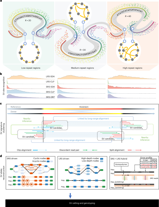
HitSV is an alignment-based SV detection approach supporting long-read, short-read and hybrid sequencing data. It addresses a long-standing limitation—alignment signals are systematically distorted in repetitive and complex regions, leading to missed, fragmented or misrepresented variants. HitSV redesigns the core stages—SV site recognition, SV signature clustering, and SV reconstruction and genotyping—by explicitly modeling the interaction between genomic repetitiveness and signature intensity (Fig. 1; Methods).

SV site recognition

HitSV adopts a repetitiveness- and signature-density-aware breakpoint recognition strategy that models SV signature densities under different degrees of local repetitiveness, using population-scale reference LRS and SRS data (40 shared samples in HPRC⁴⁶ and 1KGP⁶). It constructs empirical distributions over repeat contexts for signal types including sequence divergences, clippings and DRPs. These distributions inform rule-based, data-type-specific criteria that enable sensitive detection in repeat-rich regions where the signals are attenuated or obscured (Extended Data Fig. 1 and Supplementary Note 1).

SV signature clustering

SV-spanning reads frequently show confounded breakpoint signals, particularly in large, heterozygous or repeat-associated rearrangements. HitSV addresses these challenges through a progressive clustering strategy that treats breakpoints as latent variables inferred from SV signatures (Supplementary Fig. 1). By iteratively refining breakpoint probability distributions and integrating compatible clusters, HitSV aggregates fragmented evidence from dispersed signals and disentangles overlapping signatures from distinct alleles, enabling accurate recovery of complex events.

SV reconstruction and genotyping

HitSV performs haplotype-resolved local assembly using a unitig-centered de Bruijn graph (unitig-dBG) that integrates both variant-supporting and nonvariant reads within SV-affected regions (Supplementary Fig. 2). For short-read data, coverage-informed graph traversal generates candidate contigs beyond intrinsic read-length limits. For long-read data, HitSV constructs candidate contigs by clustering read-derived unitig-dBG paths. With hybrid data, HitSV uses long-read contigs as backbones and polishes them with short-read consensus. Candidate alleles are evaluated based on k-mer statistical modeling that realigns constituent reads to identify the most probable contig pairs for SV calling and genotyping. This approach mitigates the trade-off between conservative yet truncated allele inference and aggressive but error-prone reconstruction, enabling high-fidelity and haplotype-aware characterization of complex SVs.

Benchmarks across platforms, human cohorts and species illustrate the high yields and versatility of HitSV

We evaluated the performance of HitSV using 102 human datasets and 6 nonhuman species, namely, Macaca fascicularis⁴⁷, Mus musculus⁴⁸, Drosophila melanogaster⁴⁹, Danio rerio⁵⁰, Arabidopsis thaliana⁵¹ and Glycine max⁵², from LRS, SRS and hybrid settings. A total of 13 representative state-of-the-art SV callers were compared, including 5 LRS callers (Sniffles2 (ref. ⁵³), cuteSV2 (ref. ²²), SVDSS2 (ref. ²⁴), Sawfish⁵⁴ and SVision-pro⁵⁵), 4 SRS callers (Manta¹⁵, LUMPY¹⁶, DELLY¹⁷ and GATK-SV³), 1 hybrid caller (blend-seq⁵⁶) and 3 pangenome-informed or graph-based methods (DRAGEN³⁵, PanGenie⁵⁷, VG⁵⁸; Supplementary Tables 1 and 2).

LRS benchmarks

In the Genome in a Bottle (GIAB) HG002 benchmark with the NIST-Q100 truth (v1.1 (ref. ⁵⁹)), HitSV reached genotype F1 scores (F1-GTs) of 85.00% and 88.48% on 30× PacBio HiFi and ONT data, respectively, outperforming SOTA callers by 15.34–71.68% (Fig. 2a and Supplementary Tables 3 and 4), and the advantage becomes larger with more stringent Truvari parameters (Extended Data Fig. 2a). We further extended this benchmark to 70 LRS datasets from 35 HGSVC¹³ samples covering all five 1000 Genomes Project (1KGP) superpopulations. HitSV achieved, on average, 12.82% (PacBio) and 12.93% (ONT) higher F1-GTs than the best runner-up (Fig. 2b and Supplementary Table 5). The F1-GT on HG002 fell within the 95% prediction interval of that estimated from HGSVC, indicating consistent performance on human datasets. Moreover, HitSV demonstrated cross-species transferability. Across animal and plant genomes, HitSV achieved average F1-score advantages of 4.83–14.54% (PacBio) and 3.25–21.71 % (ONT) relative to the evaluated LRS callers (Fig. 2a and Supplementary Table 6), using the same empirical signature-distribution model.

Hybrid benchmarks

The hybrid mode is intended for settings where deep LRS becomes impractical for population-scale cohorts or nonmodel organism projects. In HG002, HitSV using 4× LRS plus 30× SRS data achieved performance comparable to or higher than Sniffles using 30× LRS alone, and outperformed blend-seq by 11.92% under the matched 4× PacBio plus 30× SRS setting (Fig. 2a and Supplementary Table 7). Similar trends were observed across the six nonhuman species, particularly for HiFi-based datasets (Fig. 2a and Supplementary Table 6). Thus, hybrid sequencing provides a cost-effective option rather than a replacement for high-depth LRS for SV discovery.

SRS benchmarks

In HG002, HitSV achieved substantially higher F1-GT than single-reference SRS callers Manta and DELLY (by 10.47% and 20.28%, respectively) and also outperformed integrated pipelines such as GATK-SV (Fig. 2a and Supplementary Tables 6 and 8). The improvement persisted in both GIAB hard and easy regions⁶⁰ (Extended Data Fig. 2b). In multispecies benchmarks, HitSV outperformed single-reference callers by 10.76–24.52% (F1 score). We also compared HitSV with three SOTA pangenome-based callers. HitSV achieved substantially higher precision. Besides contributing to new SV discovery (Supplementary Table 9), it also rescued a considerable number of false negatives (FNs) of the pangenome-based callers in pan-reference-covered regions (Methods; Fig. 2c, Supplementary Note 2 and Supplementary Table 10).

Overall, HitSV achieved high performance across long-read, short-read and benchmarked hybrid sequencing data, while substantially reducing the long-read coverage required for reliable SV discovery. Together with the affordable time cost and memory usage across species genomes and 3,202-sample 1KGP benchmarks (Supplementary Note 3 and Supplementary Tables 11 and 12), these results support its practical application in large-scale studies.

Characterization of HitSV in various contexts

We further investigated the behavior of HitSV on the HG002 benchmark in contexts of genome variation (that is, SV types, sizes and local references) and sequencing depths. Three advantages were observed.

First, HitSV has remarkable precision in SV reconstruction. In Truvari ‘refine’ mode, HitSV outperformed Sawfish in sequence-level reconstruction accuracy under all stringency thresholds (Fig. 3a and Supplementary Table 13). Specifically, the F1-GT was 96.70% for HitSV compared to 91.44% for Sawfish at 95% similarity (-p 0.95) and 83.61% for HitSV compared to 72.58% for Sawfish for perfect reconstruction (-p 1). This originates from the use of all SV-spanning reads, rather than only read segments proximal to alignment-inferred breakpoints, for assembly and allele selection.

Second, the advantages of HitSV were more pronounced for challenging genomic regions and SV types. SVs were robustly detected across highly repetitive classes including simple repeat, SINE and satellite-enriched regions, as well as in GIAB challenging medical genes (Challenging Medical Relevant Genes⁶¹; Fig. 3b and Supplementary Table 14). Furthermore, HitSV produced high yields for long (>1 kb) and very long (>5 kb) INS events, on which other callers decayed, generating more balanced yields for DEL and INS in the NIST-Q100 callset (Fig. 3c,d, Extended Data Fig. 2c,d and Supplementary Table 15). Without using a pangenome, HitSV recovered a considerable number of >1 kb insertions from short reads with high precision (169/183, 92.35%), while other de novo callers showed lower recall (Manta = 14/57, 24.56%; LUMPY = 33/190, 17.37%; DELLY = 28/176, 15.91%). Precision remained high for various levels of local repetitiveness and mappability (Supplementary Table 16), and the recovered insertions were predominantly mobile-element insertion (MEI) related (Supplementary Table 17).

Third, HitSV is robust under limited LRS depths. We downsampled HG002 LRS datasets to find that HitSV with 6× data surpassed major callers with 30× data, and, by 10× data, HitSV arrived at the saturating yield of Sawfish (Fig. 3e and Supplementary Table 18). Hybrid configurations combining low-coverage LRS (2–4×) with standard-depth SRS achieved performance comparable to, and in several cases exceeding, that of high-coverage LRS alone (Fig. 3e). Even one SV-spanning long read was often sufficient for HitSV to guide SV-allele selection (Supplementary Fig. 3), while conversely SRS data provide dense local evidence for breakpoint identification in regions insufficiently covered by long reads. Furthermore, at extreme LRS coverage (1–2×), SRS data contributed a substantial portion (27.25–42.76%) of yield (Fig. 3f and Supplementary Table 19). These results underscore HitSV’s effectiveness in handling low-depth LRS data and the benefit of joint modeling.

Finally, we characterized HitSV FN and false-positive profiles (Fig. 3g). Errors were concentrated in extremely repetitive or low-mappability contexts—FNs mainly reflected missed INS with insufficient spanning evidence, whereas false positives arose from ambiguous allele representation, repeat copy-number estimation or sparse long-read support. Similar patterns were observed in HGSVC samples (Supplementary Note 4).

Application of HitSV to large-scale genomics datasets

To evaluate HitSV in a population-scale SRS setting, we re-analyzed the 1KGP phase 4 cohort (n = 3,202; Supplementary Table 12). The resulting HitSV-SRS-callset was compared to the official 1KGP-SRS-callset generated by the combined GATK-SV, svtools and Absinthe⁶ pipeline. Across the cohort, HitSV identified 228,025 SVs, a 31.5% increase over the official 1KGP-SRS-callset. A total of 93,242 SVs were not reported in 1KGP-SRS-callset. On average, 18.3% more SVs (11,405 versus 9,639) were identified per genome, consistently across superpopulations (Fig. 4a).

We evaluated HitSV-specific SVs using various external supports. First, a matched-sample evaluation was conducted using assembly-based HPRC (matched n = 40) and HGSVC (matched n = 35) callsets as independent validation resources. In matched samples, on average, 84.90% and 85.26% of HitSV-specific SVs were corroborated by assembly-based evidence, which were 26.01% and 23.95% higher than for 1KGP-SRS-specific SVs (Fig. 4b and Supplementary Table 20). Second, at the callset level, HitSV-specific SVs showed substantially greater overlap with the independent 1KGP-LRS-callset than 1KGP-SRS-specific SVs did (39,784 versus 7,170; Extended Data Fig. 3a and Supplementary Table 21). A similar trend was observed for gnomAD-SV (60,022 versus 40,584). Because the 1KGP-LRS-callset incompletely recovers the HGSVC assembly-based callsets, the absence from this resource was not definitive evidence of false positivity (Extended Data Fig. 3b and Supplementary Table 22). Allele-frequency (AF)-stratified analyses further showed that HitSV-specific SVs had more external support than official 1KGP-SRS-specific SVs in both very rare minor allele frequency (MAF) ≤ 0.2%) and relatively common classes, although unsupported rare or singleton candidates should be interpreted cautiously (Supplementary Note 5 and Supplementary Table 23).

We examined the AF landscape of SVs, as it establishes foundations for population genetic studies. Compared to the 1KGP-SRS-callset, the HitSV-SRS-callset produced smoother and faster decaying allele count (AC) distributions, with a clearer separation between rare and common variants shown in bimodal forms (Fig. 4c). A subset of SVs classified as population specific or ultrarare in the 1KGP-SRS-callset were reassigned in the HitSV-SRS-callset as shared among superpopulations (Fig. 4d). For example, 0.29% African-specific SVs in the 1KGP-SRS-callset were observed as common (AF (ge) 0.05) in at least one other superpopulation, and 0.17% were found to be shared in all superpopulations. In addition, 1.52–2.84% population-specific SVs had their frequencies strongly elevated (Fig. 4e and Supplementary Fig. 4), and 36.6% HitSV-specific SVs were population specific, increasing population-specific SVs by 23.5–36.4% per superpopulation (Extended Data Fig. 3c).

Stratification by genomic context revealed that the largest gains achieved by HitSV occurred in repetitive regions, particularly tandem repeats (TRs; Fig. 4f). While short TRs can be reliably called from SRS data^32,62, HitSV discovered multikilobase TR expansions, extending TR unit variations to >(pm) 500 copies relative to the reference and revealing stable fractions of population-unique TR alleles (Supplementary Fig. 5). Finally, many HitSV-specific SVs were found in coding and regulatory regions (Fig. 4f). To assess functional relevance, we annotated HitSV-specific variants using seven public open resources^6,63 (Supplementary Fig. 6). More than 7,300 HitSV-specific SVs were predicted to cause loss-of-function effects; three 10–40 kb deletions unique to EUR and AFR were related to retinal dystrophy⁶⁴, spastic paraplegia and congenital hypothyroidism⁶⁵, respectively; and a 50 bp common insertion was related to primary ciliary dyskinesia by AnnotSV⁶⁶ (Supplementary Table 24).

Together, by recovering SVs missed by existing pipelines and reshaping population-level AF distributions, HitSV highlights the continued value of existing short-read resources for population genetics and disease-associated studies.

HitSV resolves genomic complex SVs (CSVs)

CSVs, characterized by clustered breakpoints and multi-event architectures, represent a major challenge for alignment-based SV callers. To assess the ability of HitSV to resolve such variants, we evaluated its performance using a curated HG002 CSV benchmark as well as two GIAB trio datasets.

The HG002 CSV benchmark contained regions having multiple SV events within 500 bp proximity⁵ in the NIST-Q100 truth set. Using LRS data, HitSV outperformed other SV callers in CSV detection (Fig. 5a,b and Supplementary Table 25). Notably, its advantage became more pronounced as CSV complexity increased. In extremely complex regions (local repetitiveness, R > 120 and >6 SVs), HitSV achieved F1-GT of 71.83%, whereas other tools consistently fell below 40%. Furthermore, when assessed by sequence accuracy (‘refine’ mode, -p 0.95), HitSV achieved 69.12–100% F1, whereas Sawfish lagged by 6.8–34.93% across CSV regions (Fig. 5c and Supplementary Table 26).

To better understand the sources of difficulty in CSV detection, we defined the following three alignment characteristics: (1) heterogeneous SV signatures, which quantify breakpoint heterogeneity by cumulative Kullback–Leibler divergence (KLD) between alignment-derived and ground-truth breakpoint distributions (Methods). Increased signature heterogeneity led to larger performance gaps between HitSV and signature-clustering methods such as Sniffles2 (Fig. 5d and Supplementary Table 27), indicating improved resilience of HitSV to breakpoint crowding and signal interference. For example, within the intron of GALNT9, HitSV correctly phased and resolved clustered SV signals, whereas other methods showed substantial discrepancies (Fig. 5e and Supplementary Fig. 7). (2) Alignment distortion—CSV regions frequently showed reduced gap-compressed identity (Fig. 5f and Supplementary Table 28), where concordant small nucleotide variations obscured single large events. In the exon of CYP4F12, HitSV recovered integral insertions with near-complete variant lengths, which were missed by others (Fig. 5g and Supplementary Fig. 8). (3) Abnormal local alignments—CSV loci often display low coverage or extensive clipping without reliable split alignments; nevertheless, HitSV retained sensitivity and reconstructed SVs from such limited evidence.

We then applied HitSV on two GIAB trio-samples’ LRS datasets to assess its generalizability. In both trios, HitSV achieved higher Mendelian consistency rates, indicating improved accuracy in a familial context (Fig. 5h and Supplementary Table 29). Its advantage was most pronounced for CSVs showing multi-allelic heterozygosity. In such cases, HitSV clustered read-derived paths according to their discrepancies in the unitig-dBG and reconstructed allelic sequences independently, while signature-clustering-based approaches commonly fail by collapsing signals into a single, incorrect SV representation. A representative case at the GSE1 gene, comprising an insertion-rich paternal allele and an insertion-deletion mixed maternal allele, is shown in Fig. 5i and Extended Data Fig. 4. HitSV uniquely reconstructed both alleles in HG002 and, concordantly, the parental haplotypes (HG003 and HG004), whereas other tools largely missed SVs or produced coarse merged calls.

Collectively, these results demonstrate that HitSV extends accurate SV detection beyond simple events to highly complex rearrangements. More examples can be found in Extended Data Fig. 5 and Supplementary Figs. 9–14.

Comprehensive panel of CSVs in 557 Chinese individuals

To interrogate the CSV landscape in human populations, we applied HitSV on the large-scale ONT sequencing resource from the China 100K Genomes Project (CHN100K⁶⁷; Methods), generating a comprehensive callset of CSVs in 557 Chinese individuals. This callset enabled systematic characterization of CSVs across a large and relatively under-represented population.

Across the cohort, HitSV identified 2,990 high-confidence CSV loci (Fig. 6a and Supplementary Table 30). A total of 95.58% CSV loci were associated with genomic TRs, where canonical alignment-based callers fail to resolve (Supplementary Fig. 15). To evaluate the added diversity and generalizability of the identified CSVs, we compared the CHN100K-CSV callset (the AF > 1% subset) with 94 haplotype-resolved contigs from 47 HPRC individuals, after strictly accounting for cohort size and technical differences (Supplementary Note 6 and Supplementary Fig. 16). This conservative comparison revealed that 10.50% compared CHN100K-CSV loci remained unsupported by HPRC (Supplementary Fig. 17).

Experimental validation of select CSV loci in six CHN100K samples provided orthogonal support for the CSV calls and the reconstructed SV contigs (Extended Data Fig. 6, Supplementary Fig. 18 and Supplementary Table 31). Based on the CHN100K–HPRC comparison, allele-level enrichment analysis further identified a smaller subset of candidates likely representing population-enriched or population-specific CSVs (Supplementary Note 6). Among shared loci, CHN100K samples also showed broader allele distributions and more extensive structural diversity than HPRC (Fig. 6b, Supplementary Fig. 19 and Supplementary Tables 32 and 33).

TR-rich CSV loci showed remarkable accumulation of mobile-element-associated sequences (54.4%, 1,554/2,857), consistent with previous observations that mobile elements frequently retrotranspose within or near TRs⁶⁸. However, our analysis further revealed the widespread occurrence of coordinated expansion or contraction of TRs and MEIs, forming TR-MEI composite arrays at 70 loci (Methods; Extended Data Fig. 7a). A total of 94.3% of such arrays were common (AF > 5%) within the cohort, rather than rare or singleton events, suggesting that these structures represent recurrent and multi-allelic forms of human CSV (Extended Data Fig. 7b and Supplementary Table 34).

Accurate resolution of TR-MEI composite arrays requires reconstruction of long, multi-allelic structures. By signal aggregation and graph-based reconstruction, HitSV captured both repeat-length variation and embedded MEI sequences (Supplementary Figs. 20 and 21). Although multiple MEI families were frequently observed (Extended Data Fig. 7c), copy number and length contribution were decoupled. While ERV1-derived and SVA-derived sequences were over-represented relative to genomic background, DNA transposons were depleted (Fig. 6c and Supplementary Table 35). This decoupling underscores the structural heterogeneity of TR-MEI arrays. Although Alu and L1 showed higher copy numbers within TR-MEI arrays, they are typically present as short internal fragments. In contrast, SVA elements, despite being less frequent, contributed disproportionately to array length due to their closer-to-full-length sizes (Extended Data Fig. 7d–f). Given the nonautonomous nature of SVA retrotransposition, their insertions more likely persisted as extended structural segments once captured within TR contexts, rather than being repeatedly fragmented and amplified. Finally, despite their modest copy numbers, TR-MEI composite arrays generate genomic length variations similar to canonical VNTR (Supplementary Fig. 22 and Supplementary Table 36), highlighting their potential contribution to structural polymorphism and phenotypic effects. Supporting this regulatory potential, TR-MEI composite arrays were frequently located in gene or gene-proximal regions (Fig. 6d and Supplementary Table 37). Representative loci illustrate that segments within composite arrays span putative exonic and promoter-associated regions or contain Alu-derived sequences overlapping predicted enhancer elements. At these loci, moderate expansion leads to ~3 copies at high ACs (19.7%), with extreme expansions reaching ~24 copies in rare cases (~0.5%), substantially amplifying regulatory sequence dosage (Fig. 6e,f and Supplementary Fig. 23).

In addition to repeat-associated CSVs, 4.41% CHN100K-CSV loci were not anchored in repetitive contexts. These loci feature compact breakpoint clusters interleaved with successive insertions and deletions within short genomic intervals (~2 kb), forming highly structured multi-allelic configurations (Fig. 6g). Extending recent long-read population studies of long-range complex structural polymorphism at functional loci^10,13, these findings capture microscale compound rearrangements, characterized by high allelic diversity and moderate-to-high ACs across the cohort, suggestive of repeated remodeling of the same genomic interval yet of much shorter spans.

Collectively, the CHN100K-based analysis using HitSV provides a population-scale view of CSV at a resolution previously inaccessible. These results reveal TR-MEI composite arrays and microscale compound rearrangements as prevalent and previously underappreciated modes of human genome variation.

Comprehensive characterization of SVs has long been a cornerstone of genomic research, yet continues to be constrained by the interplay among read length, the intrinsic complexity of the genome, and sequencing cost. The high sensitivity of HitSV can be primarily attributed to the improved signal aggregation by repetitiveness and signature density-aware site recognition and probabilistic breakpoint clustering. By reconciling weak or conflicting evidence into coherent SV hypotheses, HitSV achieved a 10.47–24.52% improvement over commonly used de novo short-read callers on both human and nonhuman datasets (F1 score/F1-GT score), demonstrating that effective modeling of alignment uncertainty can partially compensate for limited read length.

Accurate SV-allele reconstruction is critical for genotyping and downstream interpretation. HitSV used heuristic dBG path searching, clustering and merging to fully reconstruct allele-specific sequences, and outperformed SOTA long-read callers by 15.34–71.68% in F1-GT scores (HG002 benchmark). Moreover, its refined F1-GT scores reached 96.70% at 95% similarity (-p 0.95), highlighting the capability of near-complete SV reconstruction for an individual genome.

A distinctive strength of HitSV lies in its unified modeling of long-read and short-read data. Low-coverage (2–4×) long-read data ensure contig continuity and haplotype separation, whereas short-read data (30–60×) provide refined alleles and statistical evidence, resulting in a 11.92% F1-GT improvement over blend-seq and equal or higher performance than SOTA long-read callers on deep LRS data, offering a cost-effective alternative for scaling up population studies.

Application to the 1KGP cohort suggested that improved sensitivity also enables meaningful reanalysis of large cohorts, that is, a number of missed SVs can be rediscovered to reshape AF distributions across populations. Notably, variants previously regarded as population specific or ultrarare were frequently reassigned as shared at appreciable frequencies, indicating that earlier technical limitations contributed to biases in population stratification. Although the limitations of SRS remain, these results highlight that methodological advances can extend the value of legacy datasets.

Beyond generic SV discovery, HitSV enables systematic exploration of complex SVs when sufficient long reads are available. Benchmark and trio-based evaluations show improved resolution of clustered, multi-allelic and haplotype-specific rearrangements. Extending to a large Chinese cohort reveals thousands of CSV loci and uncovers structural patterns beyond canonical SV categories, including TR-MEI composite arrays and microscale compound rearrangements. The prevalence, allelic diversity and moderate-to-high population frequencies of these structures suggest that coordinated repeat instability, retrotransposition and localized sequence remodeling represent stable modes of genomic variation rather than rare mutational events.

Several limitations are noteworthy. First, extremely large or highly entangled rearrangements continue to pose challenges for local assembly-based reconstruction, while the ambiguous representation of complex alleles remains a hurdle for downstream annotation. Second, the performance of hybrid sequencing across large-scale, real-world cohorts remains to be established as such datasets emerge. Finally, the recovery of large insertions from SRS data should also be interpreted in a variant-class-specific manner because the truly new sequences remain intrinsically difficult to reconstruct from short reads. LRS or hybrid sequencing is therefore preferable for detecting large non-MEI insertions and complex insertions in highly repetitive regions. Collectively, HitSV expands the observable spectrum of structural variation, providing a valuable foundation for population genomics and the characterization of complex genetic architectures.

SV site recognition

Local repetitiveness and genome windows

The reference was divided into 600-bp-size windows with 300 bp overlaps. For each window, a measure of local repetitiveness (termed as (R)) was defined as:

where (left(l,rright)) denotes the window coordinates of the reference (s). (R) rises with local sequence repetitiveness.

SV signature collection

Multiple kinds of SV-associated signatures were collected in each window, including sequence divergence in alignments (SDAs), CLPs and DRPs (SRS only). HitSV extracts SDA, that is, significant divergences in CIGARs (single long insertions/deletions ≥ min_SV_length or dense small divergences defined as more than n (10 for LRS and 3 for SRS) mismatch/indel events occurring within a 200-bp region) and split alignments, and CLP signatures by traversing the input alignment file. DRP signatures are derived from the abnormal placements of pair-end reads implied by the alignments. All the signatures are represented as a quadruple:

where ({n}_{mathrm{SDA}}), ({n}_{mathrm{CLP}}) and ({n}_{mathrm{DRP}}) represent the numbers of SDA, CLP and DRP signatures within the window, respectively.

Signature distributions

SV signals manifest heterogeneously across sequencing technologies and genomic contexts, particularly under varying levels of local repetitiveness. Through extensive empirical inspection of long-read and short-read alignments, we observed several recurring yet poorly quantified phenomena—(1) different SV signatures dominate in long-read versus short-read data; (2) the strength of these signatures varies systematically with local repeat complexity and (3) SV-like signals occasionally appear in regions without SV events, especially within highly repetitive sequences. Furthermore, HitSV designs a model to describe the correlation between SV signatures and local repetitiveness, to distinguish true SV-supporting patterns from background noise in a principled manner.

HitSV identifies candidate SV loci using prebuilt signature distributions that quantify local signature intensity across repetitiveness levels. Separate distributions were constructed for long-read and short-read data using sequencing datasets from 40 samples shared in HPRC and 1KGP, respectively. Assembly-based ground-truth SV callsets from HPRC were used to label SV windows. Two-dimensional (repetitiveness/signature intensity) empirical distributions were then constructed for SV windows, alongside matched background distributions from non-SV windows (Extended Data Fig. 1). Also refer to Supplementary Note 1 for more detailed characterizations and discussions on the signature distributions.

SV candidate site recognition

Guided by the signature distributions, HitSV adopts a rule-based model to identify candidate SV windows. For long-read data, SV signals are dominated by SDAs and CLPs. A genome window is therefore classified as an SV candidate site if more than ({T}_{mathrm{LR}}) reads within it show either indels longer than 30 bp or clipped segments exceeding 300 bp. For short-read data, where SDAs, CLPs and DRPs jointly contribute and signal attenuation is prominent in repetitive regions, a window is recognized as candidate if any of the following conditions is satisfied: (1) (R) is higher than 40; (2) the number of SDA reads is higher than (mathrm{MAX}left({T}_{mathrm{SDA}},2right)); (3) the number of CLP reads is higher than (mathrm{MAX}left({T}_{mathrm{CLP}},2right)); and (4) the number of DRP reads is higher than (mathrm{MAX}left({T}_{mathrm{DRP}},2right)). Here the default values of ({T}_{mathrm{LR}}), ({T}_{mathrm{SDA}}), ({T}_{mathrm{CLP}}) and ({T}_{mathrm{DRP}}) are set to 10% local read depth, ensuring robustness across variable coverage while suppressing spurious signals from individual outlier reads. Using these distribution-informed rules, HitSV recovered 98.1% (LRS) and 89.2% (SRS) of HG002 SV sites (19,234 in total), demonstrating effective recall of true SV loci for downstream refinement. Moreover, it also shows generalizability by comparing the SV calls of the distribution-modeling samples with those of other 1KGP samples (Supplementary Note 7).

SV signature clustering

It is difficult to comprehensively collect all SV-associated windows and obtain a purified read set for downstream assembly, which arises because SVs may span multiple windows owing to multiple breakpoints or dispersed repeats, and signals from distinct SV events may become entangled due to heterozygosity or complex rearrangements. HitSV uses a progressive approach with two phases for refined SV signature clustering and candidate event inference.

Phase 1

HitSV infers SV breakpoints by modeling them as latent variables and constructing probability distributions from SV signatures, enabling the removal of unlikely signals and yielding purified clusters (Supplementary Fig. 1a). For SDA clustering, individual signals are assigned inferred breakpoint probability distributions—dense small-variant signals are uniformly distributed across their affected intervals, while isolated large signals are uniformly distributed within predefined length windows (default = 600 bp) centered on their indicated start and end positions. These signal distributions are then aggregated to identify a global probability peak, which defines the final inferred breakpoint. Subsequently, HitSV filters signatures by assessing whether their centroids are sufficiently close to this inferred breakpoint to ensure clustering accuracy. For CLP clustering, individual signals are assigned a uniform breakpoint probability distribution centered around their clipping bases. For DRP clustering, the breakpoint probability distribution of each signal is calculated by integrating the precomputed insert-size distribution with the orientation and distance of the corresponding paired read-ends. For CLP and DRP clusters, the final inferred breakpoint is obtained through a process similar to that of SDA clustering.

Phase 2

HitSV scans and links all the clusters by nearby regions or large signals (SDA/DRP) through a greedy approach (Supplementary Fig. 1b), enabling comprehensive window collection. This strategy handles SVs with multiple or ambiguous breakpoints and integrates windows affected by the same event. For example, inversions—typically involving two breakpoints and four windows—are grouped in a single step (Fig. 1c). This benefit is especially pronounced for dispersed repeats like MEIs (Supplementary Fig. 1). In such cases, reads align ambiguously and are hard to collect; however, proximal or linked candidate windows allow the greedy strategy to aggregate them transitively.

Haplotype-resolved local assembly for high-fidelity SV reconstruction

Read collection for local assembly

After clustering all signals of the same SV, HitSV rescans the event-affected region—extended upstream and downstream by a fixed length (default = 500 bp)—to collect all the reads, regardless of whether they contain SV signatures or not, enabling optimal local assembly.

Unitig-dBG construction

HitSV builds a unitig-dBG⁶⁹ based on k-mers from the collected reads and local reference. Each unitig records average read coverage and is classified as high depth or low depth using a threshold depending on pre-estimated sequencing depth (default ≥20% of expected depth, minimum 2). Each unitig is labeled as cyclic or acyclic after detecting cycles in the unitig-dBG. Acyclic unitigs shared with the reference are treated as anchors. Finally, all reads are decomposed into paths through the unitig-dBG for subsequent read-to-path realignment.

SRS-based SV calling

HitSV constructs candidate SV alleles through graph walking under coverage constraints (Supplementary Fig. 2).

Exhaustive (‘blind’) contig generation

The upstream and downstream anchor nodes closest to the SV are selected as the source and sink. HitSV performs depth-first search on high-depth nodes in the dBG, assigning each node a maximum visit count (default = 9). A path is accepted only if it connects source to sink and the visit counts of all traversed nodes remain below the threshold. This operation enables exhaustive contig enumeration at affordable cost through implicit coverage control.

Contig filtering

HitSV realigns all reads to the generated contigs and rejects contigs without sufficient supporting reads.

Haplotype pairing and allele inference

Remaining contigs are treated as candidate haplotypes, and, assuming diploidy, all ({n}_{mathrm{HAP}}times left({n}_{mathrm{HAP}}+1right)/2) haplotype pairs are evaluated. For each pair (left({H}_{1},|,{H}_{2}right)), HitSV computes a likelihood:

where ({D}_{R}) is pre-estimated depth, (Xleft({H}_{1},{H}_{2}right)) is the number of unmapped reads and (Yleft({H}_{1},{H}_{2}right)) represents the concordance between read and haplotype k-mer counts:

where (khbox{-}mathrm{mer}left({H}_{1},{H}_{2}right)) indicates the k-mer set of (left({H}_{1},{H}_{2}right)), ({RS}) indicates the read set and (mathrm{Count}left(khbox{-}{mathrm{mer}}_{i},left({H}_{1},{H}_{2}right)right)) and (mathrm{Count}left(khbox{-}{mathrm{mer}}_{i},{RS}right)) indicate the counts of a specific k-mer (({kme}{r}_{i})) on (left({H}_{1},{H}_{2}right)) and ({RS}), respectively. The haplotype pair having highest likelihood is selected and re-aligned to reference using KSW2 to infer SVs.

LRS-based SV detection

Each long read is represented as a path through the constructed unitig-dBG. HitSV selects the read traversing highest number of high-depth nodes as initial path, and iteratively assigns remaining reads to existing paths or builds new ones.

SDP-based read realignment

For each read, its unitig-dBG path is aligned against those of all current paths by SDP. A read supports a contig if no structural discrepancy is detected, defined as follows: if, at any SDP-anchored node (that is, flanked by SDP-matched nodes), either the gap length in two adjacent match nodes is more than 20 bp, or both allele nodes are high depth but differ in sequence.

Path updating

Reads aligned successfully refine the corresponding path by replacing low-depth nodes at SDP-anchored positions with read-derived high-depth nodes, whereas reads being rejected by all existing contigs initiate new paths. After all reads are processed, each path is converted into a contig.

Hybrid-based SV calling and polishing

When both short-read and long-read data are available, HitSV generates candidate contigs using unitig-dBG built from long and short reads, respectively. If long-read-based contigs exist, HitSV prioritizes them as backbones and uses high-accuracy short reads to improve the base-level accuracy of backbones. In detail, (1) HitSV builds an empirical 9-mer error profile by calculating the accuracy probability of all genomic 9-mers from alignments of HG002-ONT data (using the in-house script error_profile_analysis.py), using only primary alignments, and all the k-mers harboring known variants from GIAB (v4.2.1) were filtered out. (2) HitSV first identifies the positions of all low-fidelity 9-mers (error rate > 0.2) based on sequencing error profiles and homopolymer contexts in the backbone sequence, and then extracts all short reads overlapping these positions to construct multiple local consensus sequences. A representative consensus is selected based on majority short-read support. Homopolymer lengths and 9-mer sequences are subsequently corrected by comparing the selected consensus with the backbone sequence, thereby refining local sequence accuracy for downstream analysis.

Then, HitSV reassigns all short reads to polished contigs to augment support estimation by realignment. When long-read contigs are unavailable, short-read-based contigs are used as the final assemblies, and long reads are subsequently incorporated to refine genotype accuracy see ‘SV genotyping and quality control’.

SV genotyping and quality control

HitSV genotypes SVs with a probabilistic model, in which the probability is computed through an (Mtimes N) support matrix derived from read evidence, where (M) is the number of reads and (N) is the number of contigs (2 for a diploid assumption). Each element represents the probability of observing a specific read given a particular contig. For short-read data, each read is aligned to both contigs in the candidate pair, and the resulting alignment scores are transformed to construct a likelihood-based support matrix using an exponential function. For long-read data, a binary support matrix is generated by determining whether each read supports a given contig in the pair (1 indicating support and 0 indicating no support). The support matrix is used to estimate the probability for each genotype of the contig pair, and all SVs called from the contig pair are genotyped with the highest probability correspondingly. A Phred-scaled quality score is computed from the probability. Homozygous-reference calls are discarded, variants having quality lower than a predefined threshold (default = 10) are labeled LOW, and the remaining calls are marked PASS. See Supplementary Note 8 for more details.

Complex structural variation

Definition of CSV

CSVs are defined as groups of SVs that occur on the same haplotype and whose breakpoint positions lie within 500 bp of each other. Under this definition, any pair of SVs with breakpoint proximity <500 bp is merged into a larger CSV event.

HG002 CSVs benchmark

All variants in the NIST HG002 Q100 (v1.1) truth set were first partitioned into two haplotype-specific SV sets based on their genotypes. Within each set, SVs were clustered using a maximum breakpoint distance of 500 bp and a minimum SV length of 50 bp, yielding breakpoint groups corresponding to candidate CSVs. To ensure robust downstream evaluation, each breakpoint was padded by ±500 bp to account for potential uncertainty in the reported variant boundaries, and all resulting intervals were stored in BED format. These preliminary CSV intervals were then sorted and merged using bedtools, and intersected with the high-confidence benchmark regions (GRCh38_HG2-T2TQ100-V1.1_stvar.benchmark.bed) to retain only regions suitable for reliable assessment.

In total, 2,274 nonoverlapping CSV intervals were obtained for HG002, spanning approximately 3.77 Mb. Each CSV interval was classified along two dimensions, yielding nine mutually exclusive categories for evaluating the ability for CSV identification—(1) CSV complexity, defined by the number of constituent haplotype-resolved SVs (1–2, 3–6 or >6 events), and (2) local repeat complexity, measured by the local repetitiveness, (R) ((R) < 40, 40 ≤ (R) < 119 or (R) ≥ 120).

KLD

For the HG002 sample, we computed the KLD within each CSV interval to quantify the discrepancy between the observed read-alignment pattern and the expected genotype-derived breakpoint distribution. KLD was calculated in a sliding-window manner using 10 bp windows across each CSV region. For a given window, the local KLD is defined as (ptimes mathrm{log}left(frac{p}{{p}_{a}}right)+qtimes mathrm{log}left(frac{q}{{q}_{a}}right)), where (p) denotes the fraction of reads in the window that support the true breakpoint, and (q) = 1 − (P). The expected probabilities ({p}_{a}) and ({q}_{a}) are determined from the ground-truth genotype—(1) homozygous SV, ({p}_{a}=1), ({q}_{a}=0); (2) heterozygous SV, ({p}_{a}=0.5), ({q}_{a}=0.5); and (3) homozygous reference, ({p}_{a}=0), ({q}_{a}=1). To avoid zero terms, a smoothing constant of 0.01 was added to (p), (q), ({p}_{a}), ({q}_{a}) computation. The regional KLD was obtained by summing the local KLD values across all windows in the CSV interval.

Panel of CSVs in population

Population-level CSV interval from 557 ONT samples

HitSV was applied to 557 ONT samples to generate per-sample VCFs, retaining variants supported by at least two reads. For each sample, adjacent SVs with breakpoint distance <500 bp were grouped as CSVs, and the reference was partitioned into nonoverlapping 500 bp windows to record sample-specific CSV intervals and allele counts (Supplementary Note 6). Population-level ACs were computed across samples, and windows with AF ≥ 0.1% were retained. Finally, 7,939 population CSV intervals were retained by merging adjacent intervals and excluding telomeric and centromeric regions, of which 2,857 had an AC of at least 5% (refer to https://github.com/hitbc/HitSV/blob/main/cohort_csv_analysis.md).

CSV-region contigs generation and annotation

For each sample, local contigs within CSV intervals were assembled directly from BAM files. Contigs supported by at least two reads were retained. For comparison, haplotype-resolved contigs from the 47 HPRC samples (94 haplotypes) were obtained using the same approach. All contigs and corresponding reference sequences were annotated using RepeatMasker (default parameters) and tandem-repeat finder (trf input.fa 2 7 7 80 10 10 500 -h -d -ngs 1). Based on the RepeatMasker annotations, MEI categories (‘SINE’, ‘LINE’, ‘Retroposon’, ‘DNA’, ‘RC’ or ‘LTR’) were parsed for each contig (Supplementary Note 6).

MEI-array identification and annotation

For each contig, elements belonging to the dominant MEI type were sorted by genomic order, and DBSCAN clustering was performed based on MEI length and the distances across adjacent MEIs. A contig was classified as containing an MEI array if it met all the following criteria: (1) ≥3 MEI elements in the dominant cluster; (2) the s.d. of element lengths ≤20% of their mean; and (3) the s.d. of the distances ≤20% mean or ≤ 15 bp. If a CSV interval contains at least one MEI-array contig, the interval is defined as an MEI-array interval. Using this criterion, we identified a total of 89 CSV intervals containing MEI arrays. These CSV intervals were annotated with GENCODE (v44), and regulatory elements were annotated using the Ensembl regulatory feature database (GRCh38; v115; Supplementary Note 6).

Contig clustering within CSV intervals

Each CSV interval was stratified into TR-enriched and non-TR subregions based on reference sequence annotations. After splitting, the subregions of the 2,857 population CSV intervals collectively contained 4,807 CSV loci. Tandem-repeat finder-annotated repeats and RepeatMasker categories ‘simple_repeat’ and ‘satellite’ were considered as TR enriched, whereas all other annotated segments (including MEIs) were treated as non-TR. Contigs and the corresponding reference sequences were partitioned along these boundaries to generate region-specific contig sets. Within each contig set, all contigs were compared pairwisely using KSW2 (ksw_extd2_sse function) to identify structural differences ≥50 bp.

Variants were classified as TR derived (insertions attributable to TR expansion within TR-enriched regions) or non-TR (insertions involving non-TR sequence or occurring outside TR regions). Two contigs were assigned to the same cluster if no structural differences were detected or if differences were limited to TR-derived events; otherwise, they were assigned to distinct clusters. For each CSV interval, the cluster number was defined as the total number of distinct contig clusters observed.

Classification of CSV interval

Based on the aggregated variant profiles above, each subregion was assigned to one of the following categories: (1) no SV—no structural differences detected among contigs; (2) pure TR—all differences attributable solely to TR-derived insertions; (3) TR with non-TR SVs—non-TR insertions detected within TR-enriched subregions; (4) non-TR with TR SVs—TR-type insertions detected within non-TR subregions; (5) pure non-TR—only non-TR insertions present within non-TR subregions; and (6) non-TR with both types—both TR and non-TR insertions observed within non-TR subregions. These classifications were used to quantify the structural complexity of contigs within each CSV interval.

CHN100K–HPRC comparison workflow and analysis

The analytical workflow built for the SV comparison in CHN100K and HPRC callsets, including SV region filtration, downsampling analysis of SV regions and recognition of CHN100K-specific SV regions, is detailed in Supplementary Note 6.

CSV selection and experimental validation

Candidate CSV alleles for experimental validation were selected from the CHN100K population CSV callset. Candidate loci were required to be detected by HitSV in ≥1 of six CHN100K individuals whose genomic DNA samples are available, and prioritized if they were CHN100K specific, showed genotype differences between CHN100K and HPRC, or the HitSV-assembled contigs showed intersample length or sequence differences discriminable by PCR amplicon size or Sanger alignment.

Experimental feasibility assessment

Candidate loci were required to contain nonrepetitive flanking sequences on both sides of the target interval, to have an expected amplicon length compatible with PCR amplification, and to avoid extreme GC content, highly repetitive internal sequence and long homopolymer tracts. Homozygous variant loci were preferentially selected to improve target-contig amplification specificity.

Qualified loci were then validated by PCR amplification of the target intervals. PRC primers were designed for each contig using Primer3Web (v4.1.1) and are listed in Supplementary Table 38. Sample DNA was amplified using LongAmp Taq 2× Master Mix (M0287S, NEB) and the products were subjected to 1% agarose gel electrophoresis. Products were purified from the predicted bands by TIANgel Purification Kit (DP219, TIANGEN) and Sanger sequenced at Sangon Biotech. Sanger reads were aligned to the HitSV-inferred contigs and the corresponding reference sequence to confirm the amplified locus and the local CSV allele structure where technically possible.

Benchmarking methodology

Datasets and downsampling

The datasets of human and nonhuman genomes were obtained from previous studies (Supplementary Table 1). All reads were pre-aligned to the corresponding references using minimap2 (ONT), pbmm2 (PacBio) or BWA-MEM (short reads), and converted to sorted BAM files using SAMtools (Supplementary Table 2). For downsampling benchmark, the long-read datasets were downsampled to 1–10×, 15×, 20× and 25×, and the 60× short-read dataset to 15× and 30× using SAMtools.

Multispecies assembly-based benchmark sets

Recently published telomere-to-telomere (T2T) assemblies of M. fascicularis, M. musculus, D. melanogaster, D. rerio, A. thaliana and G. max, and their corresponding official reference genomes, were collected from public resources (Supplementary Table 1). For each species, we generated an assembly-based SV benchmark following the general strategy used by DeFrABB (https://github.com/usnistgov/defrabb) and the GIAB HG002 NIST-Q100 benchmark. In detail, each T2T assembly was aligned to the corresponding reference genome using minimap2, and Dipcall was used to generate SV calls and callable regions. Because only primary assembly sequences were available for the nonhuman T2T assemblies, Dipcall was run by converting such assemblies to two identical haplotypes as inputs (for example, ‘run-dipcall prefix reference.fa hap1.fa hap1.fa > prefix.mak & & make -f prefix.mak’, according to the suggestion of the pipeline). The resulting Dipcall SV VCFs and high-confidence BED files were used as the benchmark callsets and callable regions, respectively. To account for the larger divergences between species-specific assemblies and their reference genomes, minimap2 assembly-alignment presets -x ‘asm10’ or -x ‘asm20’ were evaluated when generating benchmark callsets. These presets produced benchmark sets of different sizes and stringencies, as summarized in Supplementary Table 39. The comparisons under the different ASM presets are shown in Fig. 2 and Supplementary Table 6.

HG002, HPRC and HGSVC ground truth

For HG002, the NIST-Q100 (v1.1) callset (Supplementary Table 1) from the GIAB Consortium was used as ground truth. For each of HPRC samples, the official callset composed by a DipCall-based pipeline was used as the ground truth (Supplementary Table 1). For each of the HGSVC samples, the ground truth was composed by following the same approach as for the species genomes, while the ‘-x asm5’ parameter was applied for genome alignment.

Generation pan-reference-covered SVs and HG002-specific SVs

We first collected the HPRC pangenome resources (VCF format; Supplementary Table 1) generated by the Minigraph-Cactus pipeline, and selected only insertions and deletions with a length ≥40 bp. For each selected SV, the genomic region was extended by 1,000 bp upstream and downstream to generate a raw BED file. Overlapping or adjacent intervals were then merged using bedtools ‘merge’. HG002 NIST-Q100 truth-set SVs overlapping these intervals were classified as pan-reference-covered SVs, whereas others were classified as pan-reference-uncovered, or HG002-specific, SVs. This classification was used only for stratified comparison with PanGenie, VG and DRAGEN, and not during HitSV calling.

Benchmarking configuration

For all tools, ten threads were used whenever multithreading was applicable, and default parameters were applied unless otherwise specified. On downsampled ONT and PacBio datasets, HitSV was compared with SVision-pro, Sawfish, Sniffles2, cuteSV2 and SVDSS2. cuteSV2 was run with the ‘–genotype’ option and SVision-pro with ‘–detect_mode germline’. On downsampled Illumina datasets, HitSV, Manta, DELLY and LUMPY were evaluated at 15×, 30× and 60× coverage. To match previous DRAGEN benchmarks, HitSV was additionally run on the 35× dataset used in that study. Hybrid datasets only for HitSV are generated by combining 1–10× long reads (ONT and PacBio) with 30× or 60× short reads, respectively. The metrics of blend-seq under 4× long reads (ONT and PacBio) and 30× short reads⁵⁶ were used directly for comparison. For the HG002 pangenome-informed comparison, PanGenie and VG were evaluated using the HPRC-based pangenome resources described above, and DRAGEN (v4.4) was evaluated according to its recommended short-read SV calling workflow.

Performance evaluation

For benchmarking HG002, HGSVC and HPRC samples, F1 score, sensitivity, precision and genotype concordance (GT-F1 was calculated as the product of F1 score and genotype concordance) were computed with Truvari in ‘single’ mode, considering only PASS variants, treating duplications as insertions (–dup-to-ins), and setting –sizemax to 50,000. In nonrefined mode, pctseq (-p) was set to 0 and pctsize (-P) to 0.7, 0.9 or 1.0 for benchmarking; in Truvari’s refined mode, pctseq was set to 0.7, 0.9 or 1.0 to assess the accuracy of SV-allele reconstruction. For diploid human benchmarks, F1-GT was reported when genotype information was available. For assembly-derived nonhuman species benchmarks where genotype comparison was not applicable, F1 score was reported. HG002 evaluations were restricted to the NIST high-confidence regions, whereas HGSVC, HPRC and multispecies evaluations were restricted to the corresponding callable regions of their assembly-based benchmark sets. Furthermore, for HG002, all SVs in those regions are classified by SV type (insertions and deletions), SV size and repeat context using RepeatMasker and Challenging Medical Relevant Genes annotations. For short reads, HARD and EASY regions from GIAB were also evaluated⁶⁰. For the multi‑species benchmark, Truvari’s ‘multi’ mode was used, and evaluations were restricted to the high‑confidence regions generated by the Dipcall pipeline. Before benchmarking, all VCF files were sorted, compressed and indexed using BCFtools.

Mendelian consistency evaluation

Mendelian consistency was assessed in two trios (HG002/HG003/HG004 and HG005/HG006/HG007; Supplementary Table 29) using ONT data. HitSV, Sniffles2 and cuteSV2 were evaluated. For each tool, trio callsets in a family were merged with SURVIVOR (parameters = 10 1 1 1 0 50), ignoring BND events and converting missing genotypes to homozygous reference. After sorting and indexing the resulting VCF files, Mendelian inheritance was examined using the BCFtools mendelian2 plugin.

1000 Genomes phase 4 dataset reanalysis

We ran HitSV on a computing cluster to call SVs for the 3,202 samples (Supplementary Table 1) to obtain individual VCF files. These VCFs were merged using SURVIVOR (parameters = 500 1 1 1 0 50), retaining only non-BND PASS variants. SV quality scores were re-estimated by summing across supporting samples, and variants below a size threshold (<50 bp) were removed. For each SV, AC and AF were computed using BCFtools and annotated with AnnotSV. The merged VCF was compared with the official 1000 Genomes high-coverage release using Truvari to identify new SVs.

External evaluation of HitSV-specific SVs in the 1KGP cohort

Four external high-quality SV resources, that is, HPRC (assembly-based callset for 40 samples), HGSVC (assembly-based callset for 35 samples), the official 1KGP-callset from LRS data (1KGP-LRS-callset, long-read-alignment-based callset for 975 samples) and gnomAD-SV (short-read-alignment-based callset for 63,046 samples), were used for implementing a two-level comparison to evaluate the SV specifically discovered by HitSV from 1KGP-SRS data. At the matched-sample level, we separately extracted the HitSV-specific SVs from the individual callsets of the 75 1KGP samples shared with HPRC/HGSVC. For each sample, we then directly compared the HitSV-specific SVs to the corresponding assembly-based callset to assess precision. The same processing was done for the official SRS callset of 1KGP as well.

At the population level, the four population callsets, that is, HitSV-SRS-callset, 1KGP-SRS-callset, 1KGP-LRS-callset and gnomAD-SV callset, were merged by SURVIVOR (parameters = 500 1 1 0 0 50) first. A Venn diagram was then plotted based on the merging results to compute the numbers and proportions of HitSV-specific SVs as well as 1GKP-specific SVs overlapping 1KGP-LRS-callset and gnomAD-SV. To assess the external support of SVs in various frequencies, SVs in the complete HitSV-SRS-callset and 1KGP-SRS-callset were first stratified into rare and common subsets according to their recorded MAF values, with rare SVs defined as MAF ≤ 0.2%, and common SVs defined as MAF > 0.2%. This stratification was performed before sample extraction to ensure that the frequency categories reflected the full SRS callsets. For each frequency-specific subset, SVs carried out by the 975 samples shared with the 1KGP-LRS-callset were then extracted, generating sample-matched rare and common SV callsets for both HitSV-SRS and 1KGP-SRS. The SV subsets belonging to the same MAF range were then compared with 1KGP-LRS-callset by SURVIVOR (parameters = 500 1 1 0 0 50) similarly. The same processing was also done with the 75 HPRC/HGSVC samples.

Command lines and detailed parameter settings are provided in the Supplementary Note 3.

Reporting summary

Further information on research design is available in the Nature Portfolio Reporting Summary linked to this article.

1. Middlebrooks, C. D. et al. Association of germline variants in the APOBEC3 region with cancer risk and enrichment with APOBEC-signature mutations in tumors. Nat. Genet. 48, 1330–1338 (2016).

   Article  CAS  PubMed  PubMed Central  Google Scholar 

2. Hardwick, R. J. et al. Haptoglobin (HP) and haptoglobin-related protein (HPR) copy number variation, natural selection, and trypanosomiasis. Hum. Genet. 133, 69–83 (2014).

   Article  CAS  PubMed  Google Scholar 

3. Collins, R. L. et al. A structural variation reference for medical and population genetics. Nature 581, 444–451 (2020).

   Article  CAS  PubMed  PubMed Central  Google Scholar 

4. Sudmant, P. H. et al. Global diversity, population stratification, and selection of human copy-number variation. Science 349, aab3761 (2015).

   Article  PubMed  PubMed Central  Google Scholar 

5. Sudmant, P. H. et al. An integrated map of structural variation in 2,504 human genomes. Nature 526, 75–81 (2015).

   Article  CAS  PubMed  PubMed Central  Google Scholar 

6. Byrska-Bishop, M. et al. High-coverage whole-genome sequencing of the expanded 1000 Genomes Project cohort including 602 trios. Cell 185, 3426–3440 (2022).

   Article  CAS  PubMed  PubMed Central  Google Scholar 

7. Weischenfeldt, J., Symmons, O., Spitz, F. & Korbel, J. O. Phenotypic impact of genomic structural variation: insights from and for human disease. Nat. Rev. Genet. 14, 125–138 (2013).

   Article  CAS  PubMed  Google Scholar 

8. Chiang, C. et al. The impact of structural variation on human gene expression. Nat. Genet. 49, 692–699 (2017).

   Article  CAS  PubMed  PubMed Central  Google Scholar 

9. Li, Y. et al. Pan-cancer proteogenomics connects oncogenic drivers to functional states. Cell 186, 3921–3944 (2023).

   Article  CAS  PubMed  Google Scholar 

10. Schloissnig, S. et al. Structural variation in 1,019 diverse humans based on long-read sequencing. Nature 644, 442–452 (2025).

    Article  CAS  PubMed  PubMed Central  Google Scholar 

11. Ho, S. S., Urban, A. E. & Mills, R. E. Structural variation in the sequencing era. Nat. Rev. Genet. 21, 171–189 (2020).

    Article  CAS  PubMed  Google Scholar 

12. Kosugi, S. & Terao, C. Comparative evaluation of SNVs, indels, and structural variations detected with short- and long-read sequencing data. Hum. Genome Var. 11, 18 (2024).

    Article  CAS  PubMed  PubMed Central  Google Scholar 

13. Logsdon, G. A. et al. Complex genetic variation in nearly complete human genomes. Nature 644, 430–441 (2025).

    Article  CAS  PubMed  PubMed Central  Google Scholar 

14. Rausch, T., Marschall, T. & Korbel, J. O. The impact of long-read sequencing on human population-scale genomics. Genome Res. 35, 593–598 (2025).

    Article  CAS  PubMed  PubMed Central  Google Scholar 

15. Chen, X. et al. Manta: rapid detection of structural variants and indels for germline and cancer sequencing applications. Bioinformatics 32, 1220–1222 (2016).

    Article  CAS  PubMed  Google Scholar 

16. Layer, R. M., Chiang, C., Quinlan, A. R. & Hall, I. M. LUMPY: a probabilistic framework for structural variant discovery. Genome Biol. 15, R84 (2014).

    Article  PubMed  PubMed Central  Google Scholar 

17. Rausch, T. et al. DELLY: structural variant discovery by integrated paired-end and split-read analysis. Bioinformatics 28, i333–i339 (2012).

    Article  CAS  PubMed  PubMed Central  Google Scholar 

18. Ye, K., Schulz, M. H., Long, Q., Apweiler, R. & Ning, Z. Pindel: a pattern growth approach to detect break points of large deletions and medium sized insertions from paired-end short reads. Bioinformatics 25, 2865–2871 (2009).

    Article  CAS  PubMed  PubMed Central  Google Scholar 

19. Fan, X., Abbott, T.E., Larson, D. & Chen, K. Breakdancer: identification of genomic structural variation from paired-end read mapping. Curr. Protoc. Bioinform. 45, 15.6.1–15.6.11 (2014).

    Article  Google Scholar 

20. Sedlazeck, F. J. et al. Accurate detection of complex structural variations using single-molecule sequencing. Nat. Methods 15, 461–468 (2018).

    Article  CAS  PubMed  PubMed Central  Google Scholar 

21. Heller, D. & Vingron, M. SVIM: structural variant identification using mapped long reads. Bioinformatics 35, 2907–2915 (2019).

    Article  CAS  PubMed  PubMed Central  Google Scholar 

22. Jiang, T. et al. Long-read-based human genomic structural variation detection with cuteSV. Genome Biol. 21, 189 (2020).

    Article  CAS  PubMed  PubMed Central  Google Scholar 

23. Chen, Y. et al. Deciphering the exact breakpoints of structural variations using long sequencing reads with DeBreak. Na. Commun. 14, 283 (2023).

    Article  CAS  Google Scholar 

24. Denti, L., Khorsand, P., Bonizzoni, P., Hormozdiari, F. & Chikhi, R. SVDSS: structural variation discovery in hard-to-call genomic regions using sample-specific strings from accurate long reads. Nat. Methods 20, 550–558 (2023).

    Article  CAS  PubMed  Google Scholar 

25. Lin, J. et al. SVision: a deep learning approach to resolve complex structural variants. Nat. Methods 19, 1230–1233 (2022).

    Article  CAS  PubMed  PubMed Central  Google Scholar 

26. Quenez, O. et al. Detection of copy-number variations from NGS data using read depth information: a diagnostic performance evaluation. Eur. J. Hum. Genet. 29, 99–109 (2021).

    Article  CAS  PubMed  Google Scholar 

27. Helal, A. A., Saad, B. T., Saad, M. T., Mosaad, G. S. & Aboshanab, K. M. Benchmarking long-read aligners and SV callers for structural variation detection in Oxford Nanopore sequencing data. Sci. Rep. 14, 6160 (2024).

    Article  CAS  PubMed  PubMed Central  Google Scholar 

28. Ahsan, M. U., Liu, Q., Perdomo, J. E., Fang, L. & Wang, K. A survey of algorithms for the detection of genomic structural variants from long-read sequencing data. Nat. Methods 20, 1143–1158 (2023).

    Article  CAS  PubMed  PubMed Central  Google Scholar 

29. Wu, D. et al. Large-scale whole-genome sequencing of three diverse Asian populations in Singapore. Cell 179, 736–749 (2019).

    Article  CAS  PubMed  Google Scholar 

30. Walter, K. et al. The UK10K project identifies rare variants in health and disease. Nature 526, 82–90 (2015).

    Article  CAS  PubMed  PubMed Central  Google Scholar 

31. Gudbjartsson, D. F. et al. Large-scale whole-genome sequencing of the Icelandic population. Nat. Genet. 47, 435–444 (2015).

    Article  CAS  PubMed  Google Scholar 

32. Zhang, S. et al. Genome-wide investigation of VNTR motif polymorphisms in 8,222 genomes: implications for biological regulation and human traits. Cell Genom. 4, 100699 (2024).

    Article  CAS  PubMed  PubMed Central  Google Scholar 

33. Kidd, J. M. Mobile element insertions affect human pigmentation and skin cancer risk. Nat. Genet. 56, 1546–1547 (2024).

    Article  CAS  PubMed  Google Scholar 

34. Tanudisastro, H. A., Deveson, I. W., Dashnow, H. & MacArthur, D. G. Sequencing and characterizing short tandem repeats in the human genome. Nat. Rev. Genet. 25, 460–475 (2024).

    Article  CAS  PubMed  Google Scholar 

35. Behera, S. et al. Comprehensive genome analysis and variant detection at scale using DRAGEN. Nat. Biotechnol. 43, 1177–1191 (2024).

    Article  PubMed  PubMed Central  Google Scholar 

36. Larson, D. E. et al. svtools: population-scale analysis of structural variation. Bioinformatics 35, 4782–4787 (2019).

    Article  CAS  PubMed  PubMed Central  Google Scholar 

37. Li, H. et al. A synthetic-diploid benchmark for accurate variant-calling evaluation. Nat. Methods 15, 595–597 (2018).

    Article  PubMed  PubMed Central  Google Scholar 

38. Heller, D. & Vingron, M. SVIM-asm: structural variant detection from haploid and diploid genome assemblies. Bioinformatics 36, 5519–5521 (2020).

    Article  CAS  Google Scholar 

39. Nurk, S. et al. The complete sequence of a human genome. Science 376, 44–53 (2022).

    Article  CAS  PubMed  PubMed Central  Google Scholar 

40. Bilgrav Saether, K. et al. Leveraging the T2T assembly to resolve rare and pathogenic inversions in reference genome gaps. Genome Res. 34, 1785–1797 (2024).

    Article  PubMed  PubMed Central  Google Scholar 

41. Garg, V. et al. Unlocking plant genetics with telomere-to-telomere genome assemblies. Nat. Genet. 56, 1788–1799 (2024).

    Article  CAS  PubMed  Google Scholar 

42. Phillippy, A. M., Schatz, M. C. & Pop, M. Genome assembly forensics: finding the elusive mis-assembly. Genome Biol. 9, R55 (2008).

    Article  PubMed  PubMed Central  Google Scholar 

43. Rahman, A. & Medvedev, P. Assembler artifacts include misassembly because of unsafe unitigs and underassembly because of bidirected graphs. Genome Res. 32, 1746–1753 (2022).

    Article  CAS  PubMed  PubMed Central  Google Scholar 

44. Lai, S. et al. metaMIC: reference-free misassembly identification and correction of de novo metagenomic assemblies. Genome Biol. 23, 242 (2022).

    Article  PubMed  PubMed Central  Google Scholar 

45. Chen, Y., Zhang, Y., Wang, A. Y., Gao, M. & Chong, Z. Accurate long-read de novo assembly evaluation with Inspector. Genome Biol. 22, 312 (2021).

    Article  PubMed  PubMed Central  Google Scholar 

46. Liao, W. W. et al. A draft human pangenome reference. Nature 617, 312–324 (2023).

    Article  CAS  PubMed  PubMed Central  Google Scholar 

47. Zhang, S. et al. Integrated analysis of the complete sequence of a macaque genome. Nature 640, 714–721 (2025).

    Article  CAS  PubMed  PubMed Central  Google Scholar 

48. Liu, J. et al. The complete telomere-to-telomere sequence of a mouse genome. Science 386, 1141–1146 (2024).

    Article  CAS  PubMed  Google Scholar 

49. Liu, Y.-N., Gao, J.-J., Zhuang, X.-L., Wu, D.-D. & Sun, Y.-B. Near complete assembly of Drosophila melanogaster Canton S strain genome. Nat. Commun. 17, 329 (2025).

    Article  CAS  PubMed  PubMed Central  Google Scholar 

50. Okendo, J. et al. Complete de novo assembly and re-annotation of the zebrafish genome. Preprint at bioRxiv https://doi.org/10.1101/2025.11.17.688901 (2025).

51. Kang, M. et al. The pan-genome and local adaptation of Arabidopsis thaliana. Nat. Commun. 14, 6259 (2023).

    Article  CAS  PubMed  PubMed Central  Google Scholar 

52. Zhang, A. et al. A telomere-to-telomere genome assembly of Zhonghuang 13, a widely-grown soybean variety from the original center of Glycine max. J. Crop Sci. 12, 142–153 (2024).

    CAS  Google Scholar 

53. Smolka, M. et al. Detection of mosaic and population-level structural variants with Sniffles2. Nat. Biotechnol. 42, 1571–1580 (2024).

54. Saunders, C.T. et al. Sawfish: improving long-read structural variant discovery and genotyping with local haplotype modeling. Bioinformatics 41, btaf136 (2025).

55. Wang, S. et al. De novo and somatic structural variant discovery with SVision-pro. Nat. Biotechnol. 43, 181–185 (2025).

    Article  CAS  PubMed  Google Scholar 

56. Magner, R. Blended length genome sequencing (blend-seq): combining short reads with low-coverage long reads to maximize variant discovery. Preprint at bioRxiv https://doi.org/10.1101/2024.11.01.621515 (2025).

57. Ebler, J. et al. Pangenome-based genome inference allows efficient and accurate genotyping across a wide spectrum of variant classes. Nat. Genet. 54, 518–525 (2022).

    Article  CAS  PubMed  PubMed Central  Google Scholar 

58. Hickey, G. et al. Genotyping structural variants in pangenome graphs using the vg toolkit. Genome Biol. 21, 35 (2020).

    Article  PubMed  PubMed Central  Google Scholar 

59. Dwarshuis, N. et al. The GIAB genomic stratifications resource for human reference genomes. Nat. Commun. 15, 9029 (2024).

    Article  CAS  PubMed  PubMed Central  Google Scholar 

60. Krusche, P. et al. Best practices for benchmarking germline small-variant calls in human genomes. Nat. Biotechnol. 37, 555–560 (2019).

    Article  CAS  PubMed  PubMed Central  Google Scholar 

61. Wagner, J. et al. Curated variation benchmarks for challenging medically relevant autosomal genes. Nat. Biotechnol. 40, 672–680 (2022).

    Article  CAS  PubMed  PubMed Central  Google Scholar 

62. Cui, Y. et al. A genome-wide spectrum of tandem repeat expansions in 338,963 humans. Cell 187, 6411–6412 (2024).

    Article  CAS  PubMed  PubMed Central  Google Scholar 

63. Chen, S. et al. A genomic mutational constraint map using variation in 76,156 human genomes. Nature 625, 92–100 (2024).

    Article  CAS  PubMed  Google Scholar 

64. Bandah-Rozenfeld, D. et al. Mutations in IMPG2, encoding interphotoreceptor matrix proteoglycan 2, cause autosomal-recessive retinitis pigmentosa. Am. J. Hum. Genet. 87, 199–208 (2010).

    Article  CAS  PubMed  PubMed Central  Google Scholar 

65. Heinen, C. A. et al. Mutations in IRS4 are associated with central hypothyroidism. J. Med. Genet. 55, 693–700 (2018).

    Article  CAS  PubMed  PubMed Central  Google Scholar 

66. Geoffroy, V. et al. AnnotSV: an integrated tool for structural variations annotation. Bioinformatics 34, 3572–3574 (2018).

    Article  CAS  PubMed  Google Scholar 

67. Jiang, T. et al. A comprehensive genetic variant reference for the Chinese population. Sci. Bull. (Beijing) 69, 3820–3825 (2024).

    Article  PubMed  Google Scholar 

68. Cordaux, R. & Batzer, M. A. The impact of retrotransposons on human genome evolution. Nat. Rev. Genet. 10, 691–703 (2009).

    Article  CAS  PubMed  PubMed Central  Google Scholar 

69. Zerbino, D. R. & Birney, E. Velvet: algorithms for de novo short read assembly using de Bruijn graphs. Genome Res. 18, 821–829 (2008).

    Article  CAS  PubMed  PubMed Central  Google Scholar 

70. Li, G. et al. HitSV call results for ‘Structural variant detection across sequencing technologies’. Zenodo https://doi.org/10.5281/zenodo.22106614 (2026).

71. Li, G. et al. HitSV v2.0.4: structural variant detection across sequencing technologies. Zenodo https://doi.org/10.5281/zenodo.22230307 (2026).

Download references

Author notes

1. These authors contributed equally: Gaoyang Li, Yadong Liu

Authors and Affiliations

1. Center for Bioinformatics, Faculty of Computing, Harbin Institute of Technology, Harbin, China

   Gaoyang Li  (李高阳), Yadong Liu  (刘亚东), Anqi Zhang  (张安琪), Xiaoyi Lin  (林枭熠), Zheng Hu  (胡铮), Bo Liu  (刘博) & Yadong Wang  (王亚东)

2. Key Laboratory of Biological Big Data, Ministry of Education, Harbin Institute of Technology, Harbin, China

   Gaoyang Li  (李高阳), Yadong Liu  (刘亚东), Anqi Zhang  (张安琪), Xiaoyi Lin  (林枭熠), Zheng Hu  (胡铮), Bo Liu  (刘博) & Yadong Wang  (王亚东)

3. Center for Quantitative Biology, Academy for Advanced Interdisciplinary Studies, Peking University, Beijing, China

   Long Qian  (钱珑)

Contributions

Y.W. designed and supervised the research. G.L. and B.L. developed the algorithm and software. B.L., L.Q. and Y.L. contributed to data interpretation. G.L., A.Z. and X.L. performed algorithm benchmarking. L.Q., Y.L., G.L. and A.Z. contributed to the 1KGP4 reanalysis and CHN100K analyses. Z.H. conducted the experimental validation. L.Q., B.L. and Y.L. wrote the paper with input from all other authors. All authors read and approved the final paper.

Corresponding authors

Correspondence to Bo Liu  (刘博), Long Qian  (钱珑) or Yadong Wang  (王亚东).

Competing interests

All authors declare no competing interests.

Peer review information

Nature Biotechnology thanks Ramakrishnan Rajagopalan, who co-reviewed with Tejas Jammihal; Danny Miller; and the other, anonymous, reviewer(s) for their contribution to the peer review of this work.

Open Access This article is licensed under a Creative Commons Attribution-NonCommercial-NoDerivatives 4.0 International License, which permits any non-commercial use, sharing, distribution and reproduction in any medium or format, as long as you give appropriate credit to the original author(s) and the source, provide a link to the Creative Commons licence, and indicate if you modified the licensed material. You do not have permission under this licence to share adapted material derived from this article or parts of it. The images or other third party material in this article are included in the article’s Creative Commons licence, unless indicated otherwise in a credit line to the material. If material is not included in the article’s Creative Commons licence and your intended use is not permitted by statutory regulation or exceeds the permitted use, you will need to obtain permission directly from the copyright holder. To view a copy of this licence, visit http://creativecommons.org/licenses/by-nc-nd/4.0/.

Reprints and permissions