Category: learning

Genetic perturbation modeling aims to predict the transcriptomic impact of inhibiting or activating one or more genes, with the potential to enable scalable in silico screens for therapeutic target discovery. Recent studies have questioned whether transcriptome-level perturbation modeling is viable. Ahlmann-Eltze et al. reported that deep learning models do not outperform uninformative baselines across multiple datasets¹. Likewise, several independent benchmarks have found that a simple ‘mean baseline’, the average perturbed gene expression profile in the training set, often matches or surpasses state-of-the-art models on metrics such as mean absolute error (MAE), mean squared error (MSE) or the correlation of control-referenced deltas (Pearson(Δ_ctrl))^2,3,4,5,6,7.

In earlier work, we identified two artifacts that explain why the mean baseline can appear predictive despite lacking a perturbation-specific signal⁸. The first, control bias, arises when systematic differences between control and perturbed cells inflate control-referenced correlation metrics, a phenomenon also recently described by Viñas Torné et al.². The second, signal dilution, occurs when error metrics dilute meaningful biological signals arising from perturbations with a small but significant number of differentially expressed genes (DEGs), causing mean predictions to appear accurate. Together, these effects allow uninformative predictors to achieve deceptively high scores even when they fail to capture underlying biology, highlighting the need to evaluate whether common benchmarking metrics can distinguish uninformative from meaningful predictions in the first place. In experimental biology, positive and negative controls provide a direct means to test this. However, while the mean baseline serves as an intuitive negative control, existing benchmarks typically lack a corresponding positive control, leaving ambiguity when models perform poorly; low scores may reflect either genuine model failure or insufficient metric sensitivity.

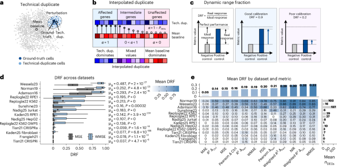
Previously, we proposed the technical-duplicate baseline as a positive control, in which one half of the cells from each perturbation are used to predict the other⁸ (Fig. 1a). Because both halves share the same perturbation-specific signal, this baseline was expected to outperform uninformative predictors such as the mean baseline. However, when we measured the performance of these baselines on the Norman19 and Replogle22 K562 genome-wide Perturb-seq (GWPS) datasets using MSE and Pearson(Δ_ctrl), we observed mixed results. As expected, the technical duplicate outperformed the mean baseline in Norman19 (Extended Data Fig. 1a,c). In Replogle22 K562 GWPS, however, it performed comparably under Pearson(Δ_ctrl) (Extended Data Fig. 1d) and underperformed on MSE (Extended Data Fig. 1b), both on average and in approximately 95% of perturbations individually (Extended Data Fig. 1e). In our subsequent analysis (detailed in Supplementary Note 1), we traced this discrepancy back to signal dilution; for Replogle22 K562 GWPS, there were only 3.25 DEGs per perturbation on average (versus 102.09 for Norman19) (Supplementary Table 1). Because the mean baseline is a better estimate of unperturbed gene expression versus the technical duplicate (largely because of greater statistical power), it displays more robust performance in datasets that have weaker perturbations on average.

Motivated by this observation, we introduce an interpolated duplicate baseline that combines the strengths of both approaches by predicting a value between the mean baseline and the technical duplicate, using an interpolation parameter α derived from the DEG P value for each gene (Fig. 1b and Extended Data Fig. 2). Predictions for strongly affected genes are dominated by the technical duplicate, whereas predictions for weakly affected genes are dominated by the mean baseline, yielding consistently positive performance (Extended Data Fig. 3).

With our positive control (interpolated duplicate) and negative control (mean baseline) in hand, we next defined a meta metric to quantify the calibration of benchmarking metrics. We term this quantity the ‘dynamic range fraction’ (DRF), which measures, for each perturbation, how effectively a metric distinguishes positive from negative controls. For any metric m(⋅), DRF is defined as

where ({hat{y}}_{n}) is the mean baseline (or any other negative control), ({hat{y}}_{p}) is the interpolated duplicate (or any other positive control), y represents the ground truth and, hence, yields perfect performance on the metric (for example, MSE = 0 or Pearson(Δ_ctrl) = 1) and ϵ is a small constant added for numerical stability. DRF captures the fraction of the theoretical dynamic range ([m(y)-m({hat{y}}_{n})]) (‘ideal response’) that is realized by the empirical range ([m({hat{y}}_{p})-m({hat{y}}_{n})]) (‘real response’) (Fig. 1c). When the positive control outperforms the negative control (and, hence, the metric is better calibrated), DRF values increase in proportion. In a miscalibrated scenario, DRF values approach zero, reflecting limited metric sensitivity to detect improvements over the negative control.

We applied DRF to assess the calibration of MSE and Pearson(Δ_ctrl) in the Replogle22 K562 GWPS and essential gene datasets⁹. In both datasets, most perturbations show low DRF values for these metrics (Extended Data Fig. 4a). Consistent with this, SP2 transcription factor (TF) inhibition in Replogle22 K562 GWPS has DRF(MSE) near zero (Extended Data Fig. 4b), yet gene set enrichment analysis (GSEA) of DEG ranks induced by SP2 perturbation recovers SP2 binding targets among the top ENCODE/ChEA gene sets (Extended Data Fig. 4c). A similar pattern was observed across multiple other TFs (that is, DRF(MSE)) near zero despite the presence of meaningful biological signal; Extended Data Fig. 4d and Supplementary Note 1, supporting the notion of signal dilution as a failure mode of MSE.

If signal dilution drives poor calibration, metrics that emphasize perturbation-specific effects should recover higher DRF. We previously proposed weighted MSE (WMSE)⁸ for exactly this purpose; WMSE upweights errors on genes with stronger perturbation effects, even when they comprise a small fraction of the transcriptome and, when used as a training objective, WMSE can increase perturbation model output variance and improve performance relative to standard MSE. As expected, WMSE displayed improved calibration relative to MSE, both for individual TF perturbations (Extended Data Fig. 4b) and at the dataset level, even in datasets with few DEGs per perturbation (Fig. 1d and Extended Data Fig. 4E).

Extending this analysis to 18 metrics spanning complementary objective families—direct reconstruction error, reference-based delta metrics and retrieval-based metrics—we found that widely used metrics such as MSE and Pearson(Δ_ctrl) are often poorly calibrated, unless evaluated in datasets with stronger perturbation strength overall, such as Norman19 (Fig. 1e). In contrast, weighted and rank-based metrics—including WMSE, weighted ({R}_{Delta }^{2}) (same weights as WMSE⁸) and normalized inverse rank (NIR)—consistently exhibited higher calibration across datasets, reflecting their shared design principle of emphasizing perturbation-specific signal. Likewise, filtering for the top 100 DEGs per perturbation also increased metric calibration in general (Extended Data Fig. 5).

To evaluate the reliability of our calibration approach, we analyzed the impact of changing the positive and negative controls for DRF calculation, the number of cells per perturbation, sequencing depth per cell or the number of highly variable genes (HVGs) selected and evaluating the relationship between perturbation strength and baseline performance (Supplementary Note 2). Compared to typical benchmarking metrics such as MSE and Pearson Δ_ctrl, we found that well-calibrated metrics (for example, WMSE, weighted ({R}_{Delta }^{2}) and NIR) amplify perturbation-specific signal and maintain higher calibration, even when data quality is lower (that is, lower library size or cell count), perturbations are weaker or selected genes have lower variance on average. Taken together, our analysis reinforces the validity of our calibration framework and utility of the well-calibrated metrics identified here.

We then used our well-calibrated metrics to measure model performance on the unseen genetic perturbation prediction task, in which models predict responses to individual perturbations held out during training (Fig. 2a, left). Nine models were evaluated: scGPT¹⁰, GEARS¹¹, PRESAGE¹², scLambda¹³, CellFlow¹⁴ and four foundation model embedding probes (fMLPs) using Geneformer¹⁵, ESM2 (ref. ¹⁶), scGPT and GenePT¹⁷ embeddings. Models span multiple generations of perturbation modeling—helping disentangle the contributions of metric calibration and model development—and we used an MLP probe to evaluate the relative utility of various foundation model embeddings for providing useful perturbation representations. Baselines include the mean baseline, control baseline (average of control cells) and a linear baseline introduced previously¹ that involves performing principal component analysis (PCA) on the training set gene expression matrix and fitting a linear model to predict unseen genetic perturbation responses using these features.

In Replogle22 K562, earlier models (scGPT and GEARS) do not outperform baselines under poorly calibrated metrics such as MSE and Pearson(Δ_ctrl) (Extended Data Fig. 6a,b), consistent with prior benchmarks^1,2,4,5,7. Under well-calibrated metrics, however, even these earlier models mostly outperform uninformative baselines (Fig. 2b–d and Extended Data Fig. 6c), suggesting that their perturbation-specific signal was present but obscured by metric choice. More recent models (PRESAGE and scLambda) go further, often outperforming uninformative baselines even under poorly calibrated metrics; indeed, on every metric, at least one deep learning model outperforms all baselines (Supplementary Table 2). These findings were also replicated in the independent Nadig25 HepG2 dataset¹⁸ (Extended Data Fig. 7 and Supplementary Table 2).

Using our fMLP probe, we also observed consistent differences in performance between perturbation embedding features, with GenePT and ESM2-based fMLP models proving more predictive overall. These results were found to be consistent across a size ablation study in which we reduced fMLP model capacity to approximately one half and one quarter of the original parameter count and trained in the Replogle22 K562 (Extended Data Fig. 7).

We next evaluated model performance on the unseen combination prediction task, in which models must predict the transcriptomic response to pairs of perturbed genes after training on each single genetic perturbation and 25% of all combos (Fig. 2a, right).

We first benchmarked on Norman19, the most widely used dataset for this task^{1,2,3,4,5,7,19}, which comprises 100 single and 124 combo (two-gene) perturbations. The additive baseline (predicts combination effects by summing single effects) performed strongly here, as expected, given that approximately 96% of effects were additive¹ and the training set covered only 31 of 4,950 possible pairs (0.63%) (these 31 pairs represent half of the total 62 combinations in our train–validation split; in contrast, the previous study¹ used all 62 combinations for training as their benchmark did not include a validation set), leaving little opportunity to learn nonadditive interactions. Most models exceeded mean and control baselines across metrics but the additive baseline remained difficult to surpass (although deep learning models outperformed it on six of 18 metrics). Further analysis shows that the additive baseline captured ~88% of the ideal performance gap in the best-calibrated metrics (Extended Data Fig. 8), comparable to the interpolated duplicate, which has access to held-out combination data. This evidence of additive baseline saturation, together with limited combinatorial coverage, suggests a limit to Norman19’s value for benchmarking models that aim to learn nonadditive genetic interactions and we recommend that future studies refrain from using this dataset as the sole benchmark of combinatorial perturbation modeling.

To test whether models can surpass additivity when exposed to a greater proportion of the combinatorial landscape during training, we evaluated Wessels23 (ref. ²⁰), which includes 28 single genetic perturbations and 157 unique perturbation pairs (training set covers 10.3% of possible combinations versus 0.63% in Norman19). In this setting, multiple models outperformed the additive baseline under WMSE and weighted ({R}_{Delta {rm{ctrl}}}^{2}) (Fig. 2e,f), and PRESAGE exceeded it on 15 of 18 metrics (Supplementary Table 2), including Pearson(Δ_ctrl) (Fig. 2g). Notably, PRESAGE is a more recent architecture that was developed after the benchmarking studies that established the additive baseline as a robust predictor compared to other models, exemplifying improving trends in model performance over time in this task. Together, these findings demonstrate that deep learning models can outperform the additive baseline when combinatorial coverage is sufficient.

Our benchmarking revealed that model performance varies substantially across datasets, reflecting differences in task difficulty. Replogle22 K562 and Nadig25 HepG2 pose a challenging unseen genetic perturbation task with weaker perturbations on average (median number of DEGs: one for Replogle22 K562 and zero for Nadig25 HepG2), whereas Wessels23 involves an unseen combination task with stronger perturbations (median number of DEGs: eight) (Supplementary Table 1). Consistent with this, positive control baselines achieve higher scores on Wessels23 than on Replogle22 K562 across all comparable metrics (Supplementary Table 2) and most models show the same pattern, indicating that performance differences across datasets largely track task difficulty rather than model-specific failure modes.

Our results also show that models exhibit substantial variation across metric families and we caution against treating any single well-calibrated metric as definitive (as discussed for complementary metric families below). For example, scGPT achieves the lowest WMSE among all models in Replogle22 K562 (0.027 ± 0.001) and highest Pearson(Δ_ctrl) on DEGs (0.367 ± 0.009) yet performs poorly on Pearson(Δ_pert) across all genes (0.081 ± 0.003) (Supplementary Table 2), barely above the mean baseline.

We also evaluated whether model performance corresponds to recovery of biological insights through an analysis of two downstream tasks: (1) pathway recovery—correlation between GSEA calculated on predicted and ground-truth perturbation effects, which is relevant to pathway analysis from model predictions, and (2) neighborhood-structure recovery—rank-based similarity between KNN graphs constructed from predicted and observed perturbation shifts, which is relevant to perturbation network analysis. Across datasets, models performing strongly under well-calibrated metrics also showed better pathway recovery (Extended Data Fig. 9a–d), with pathway recovery rankings and well-calibrated metric rankings being correlated (Replogle22 K562 ρ_avg = 0.76; Wessels23 ρ_avg = 0.84). Neighborhood recovery showed a similar but more variable pattern (Replogle22 K562 ρ_avg = 0.77; Wessels23 ρ_avg = 0.58), with the strongest correspondence between neighborhood-structure recovery and retrieval-based NIR/PDS metrics (ρ > 0.78 in all cases), consistent with their related objectives (Extended Data Fig. 9e–h). These results indicate that well-calibrated metrics capture biologically meaningful differences between models relevant to downstream analysis objectives.

In summary, we found that models frequently outperform uninformative baselines under well-calibrated metrics. This includes earlier models such as scGPT and GEARS, whose perturbation-specific signal was present but obscured by metric choice (Extended Data Fig. 6), and newer models spanning diverse architectures—including PRESAGE (attention-based, prior knowledge embeddings), scLambda (variational autoencoder) and CellFlow (flow matching)—which stand out for their stronger performance relative to uninformative baselines in these metrics. Earlier benchmarking studies had a constructive role in surfacing modeling limitations that these and other architectural advances have begun to address. In our results, PRESAGE is notable both for its strong performance and sophisticated perturbation representation approach based on biological prior knowledge. Concurrently, an independent preprint by Cole et al. systematically benchmarked foundation model and prior-knowledge-based embeddings for perturbation response prediction²¹. Their work reached complementary conclusions, showing that embeddings encoding prior knowledge can improve prediction, further underscoring the value of prior knowledge for building informative representations of genetic perturbations.

The DRF calibration framework we introduce here is not tied to a prescriptive definition of positive or negative controls; instead, it provides a general approach for assessing metric sensitivity relative to any reasonably defined performance baselines. Moreover, this framework does not eliminate the need for complementary benchmarking metrics; direct error, reference-based, weighted and retrieval-based metrics each capture distinct aspects of model behavior and should be combined in holistic model evaluations. For instance, direct error metrics are a useful guardrail against rewarding implausible model predictions, as recently demonstrated in the Virtual Cell Challenge²². That being said, we recommend MSE as it showed better calibration overall compared to MAE (Fig. 1e and Extended Data Fig. 5). In practice, a model performing substantially below baselines on either metric would warrant scrutiny regardless of calibration as this may indicate a lack of modeling realism.

Several limitations remain for this work. First, we focused on the unseen genetic perturbation and unseen combination prediction tasks, leaving the unseen context task (predicting responses in unobserved cell types, donors or conditions) unaddressed. Additionally, the contrast between Norman19 (0.63% of the combinatorial search space in training) and Wessels23 (10.3%) suggests that training set characteristics may influence the performance of both baselines and models; evaluating additional combinatorial datasets will help to characterize this relationship more thoroughly. Lastly, as the field continues to evolve rapidly, conclusions drawn from any fixed set of models necessarily reflect a snapshot of perturbation response modeling and available perturbation datasets at a particular time. Benchmarks should incorporate both earlier and up-to-date architectures to track whether advances in modeling translate to increased performance in well-calibrated benchmarks.

Overall, our findings reframe the debate on the feasibility of genetic perturbation modeling. A key obstacle has been the reliance upon uncalibrated benchmarks that obscure true model performance. With calibration-aware evaluation, we show that models can outperform uninformative baselines, contextualizing prior reports of model underperformance and helping to establish a more optimistic foundation for genetic perturbation modeling.

Baseline definition

To evaluate metric calibration and model performance, we define both uninformative and trivial baselines, along with idealized positive control baselines.

Control baseline

Computed at the dataset level, the control baseline μ_c is the averaged expression profile of 8,192 random unperturbed control cells.

Mean baseline

Computed at dataset level, it is defined as the average of averages of all train perturbations. Mathematically, given a set of M train perturbations each represented by a set of cells ({mathcal {S}}_{1},{mathcal{S}}_{2},ldots ,{mathcal {S}}_{M}) that can vary in size, the mean baseline is computed as follows:

where x_i,j represents the expression profile of the jth a cell of the ith perturbation. Note that this computation is dense and weights every perturbation equally instead of every cell equally.

Technical duplicate

The technical-duplicate baseline is defined by randomly dividing the cell set ({{mathcal{S}}}_{i}) associated with perturbation p_i in two: a ground-truth set ({mathcal {S}}_{i,mathrm{GT}}) and a technical-duplicate set ({mathcal {S}}_{i,mathrm{TD}}). The average profiles of both sets μ_i,GT and μ_i,TD are then considered the ground-truth and technical-duplicate values for evaluation, respectively. This definition aims to provide an idealized estimate of good performance where the prediction errors are only because of the inherent variability of the experiment. In other words, it answers the following question: If we were to sequence additional cells from the same perturbed biological samples (as in a technical replicate), how predictive would those new cells be of the perturbation effect observed in the original cells? Note that the technical-duplicate baseline matches the sampling of the ground truth and, hence, has limited estimation power when the original number of cells per perturbations is low. Additionally, to avoid any data leakage, all cells selected as technical duplicates are excluded from DEG computations to derive evaluation metric weights or masks and, thus, are treated as an independent duplicate dataset at evaluation time.

Interpolated duplicate

Defined at the perturbation level, the interpolated duplicate μ_i,ID is a per-gene interpolation between the technical-duplicate prediction μ_i,TD and the mean baseline prediction μ_all. Mathematically,

where α is a vector encoding DEG significance and ⊙ denotes the element-wise product operation between vectors. We define α = 1 − P_DEGs per perturbation with the help of the P values of an independent DEG analysis performed only on the held-out technical-duplicate set. This choice yields interpolation weights naturally bounded in [0, 1] and provides an interpretable confidence-like measure of whether a gene is perturbed. In other words, α reflects the strength of statistical evidence that a gene is affected by a given perturbation.

If a gene k is significantly affected by a perturbation, its associated interpolation value will be α[k] ≈ 1. Conversely, if a gene is unaffected by a perturbation, its associated value will be α[k] ≈ 0. This setup allows the interpolated duplicate to use the predictions from the technical duplicate when there is evidence that a gene changed significantly because of a perturbation while also using the estimations of the mean baseline when the gene is unaffected.

Linear baseline

Defined at the perturbation level, the linear baseline is computed as previously described¹ with its original hyperparameters. In short, we perform a PCA to obtain the principal component matrix G from the pseudobulked train dataset Y_train. We then define the matrix P as the row selected matrix corresponding to the train perturbations and find the square matrix W as

through ridge optimization with b the vector of row means of Y_train. To perform predictions for unseen perturbations, we compute

Where (tilde{P}) is the row selected version of G for the desired unseen perturbations. This baseline is defined only for the unseen single perturbation task and evaluated the performance of a deliberately simple model for the task.

Additive baseline

Defined at the perturbation level, this baseline is computed for the unseen combination task following the previous study¹. For two training perturbations μ_a and μ_b, their additive baseline prediction is given by

Data

Datasets

We compiled a diverse set of 14 genetic perturbation datasets coming from nine studies spanning ten different cell lines under activation and repression perturbations. Detailed metadata can be found in Supplementary Table 1. Datasets were obtained from the scPerturb²⁴ standardized data resource when available, as well as from the Zenodo, Figshare or Gene Expression Omnibus records for datasets not processed by scPerturb.

Processing

For every dataset, we filter out any perturbation with fewer than 12 measured cells, any cell with fewer than 200 expressed genes and any gene expressed in fewer than three cells. We use standard library size normalization (target sum of 10,000) and log1p transformation (natural logarithm) from scanpy²⁵. To balance the datasets, we enforce a maximum number of cells per perturbation calculated as the mean of cells per perturbation after previous filters were applied (Supplementary Table 1). We further select a distinct gene set per dataset composed by the union of the top 8,192 HVGs (scanpy’s sc.pp.highly_variable_genes) plus all perturbed genes.

Next, to construct our technical-duplicate ({mathcal{S}}_{TD}) and ground-truth ({mathcal{S}}_{mathrm{GT}}) sets, we perform a single random cell-wise split for every perturbation in the dataset before cross-validation. This split is fixed across folds. Subsequent train, validation and test splits are performed at the perturbation label level. For perturbations assigned to the training set, both ({{mathcal{S}}}_{mathrm{GT}}) and ({mathcal{S}}_{mathrm{TD}}) cells are available during model fitting (that is, no cell-level withholding occurs within training perturbations). For perturbations assigned to the test set, models never observe either ({{mathcal{S}}}_{mathrm{GT}}) or ({mathcal{S}}_{mathrm{TD}}) cells during training. During evaluation, only the ground-truth half ({{mathcal{S}}}_{mathrm{GT}}) of test perturbations is used as the true target, while ({mathcal{S}}_{mathrm{TD}}) is used exclusively for baseline construction (for example, technical and interpolated duplicates). This design ensures that the technical or interpolated duplicate task of predicting one half of the data from the other half is mirrored in model evaluation without introducing data leakage across cross-validation folds.

Lastly, we compute DEGs for every perturbation with respect to all other perturbed cells (excluding controls) using a t-test with overestimation of variance from scanpy’s sc.tl.rank_genes_groups. For each perturbation p_i, we perform DEG analysis separately for ({mathcal{S}}_{{i},{mathrm{GT}}}) and ({mathcal{S}}_{i,mathrm{GT}}) against all other perturbed cells in the dataset. DEG results from the technical-duplicate half (({mathcal{S}}_{i,mathrm{TD}})) are used only for constructing the interpolated duplicate as previously mentioned. DEG results from the ground-truth half (({mathcal{S}}_{i,mathrm{GT}})) are used only for weighted evaluation metrics such as the WMSE⁸. This ensures no leakage of evaluation metric weights into the construction of the interpolated duplicate. We follow the approach of a previous study⁸ by computing DEGs with all other perturbed cells as the reference instead of the control population, which ensures that we evaluate over genes that make a perturbation unique and safeguards against genes changing systematically for all perturbations. The resulting processed datasets are homogeneous in terms of experimental conditions containing a single cell line and perturbation type. The only exception to the above protocol is Replogle22 K562 GWPS, in which we randomly subsampled perturbations to 2,500 because of memory constraints.

Metric calibration assessment

We numerically define metric calibration for any functional metric (m(hat{y})) that operates on a prediction (hat{y}) and ground truth y with respect to positive and negative control predictions ({hat{y}}_{p}) and ({hat{y}}_{n}), respectively. Our proposed measure, the DRF, evaluates how much of the ideal performance gap between the perfect prediction and a negative control (m(y)-m({hat{y}}_{n})) is covered by the real performance gap between the positive control and negative control (m({hat{y}}_{p})-m({hat{y}}_{n})). Mathematically,

with ϵ being a small value for numerical stability. Note that the DRF is defined for every perturbation individually, which allows the study of different factors influencing calibration. For this work, we choose the following ground truths and controls when evaluating metric calibration:

Metrics

Because different downstream applications of perturbation models depend on distinct aspects of predictive accuracy, we assessed calibration and model performance using 18 evaluation metrics spanning complementary categories. All evaluation metrics were computed on perturbation-level pseudobulk expression profiles, ensuring comparability across models and baselines that do not generate single-cell predictions.

Direct error metrics

We measured direct reconstruction error using MSE and MAE, two metrics widely used in prior benchmarking studies (along with variants such as the root MSE)^2,3,5,26. To increase sensitivity to perturbation-specific signal, we also evaluated weighted error metrics as described in our prior work⁸. Weighted error metrics, WMSE and weighted MAE, apply gene-level weights derived from differential expression, thereby emphasizing errors in genes strongly affected by a perturbation. Whereas unweighted error metrics primarily reflect global transcriptome reconstruction accuracy, weighted error metrics emphasize errors in niche, biologically informative genes, which may be more aligned with applications such as predicting perturbation responses within particular pathways or gene modules.

Reference-based delta metrics

We also assessed relative error using reference-based delta-based metrics, which compare the predicted and observed shifts in gene expression induced by a perturbation. These were generated by combining a similarity function (Pearson correlation or the coefficient of determination R²) with a reference baseline (the mean of the control population μ_c or the perturbed mean baseline μ_all)^2,8.

For Pearson Δ, special care is required when the reference baseline coincides with the predictor being evaluated, as the metric is then undefined by construction (for example, Pearson Δ_ctrl for the control baseline, in which case the prediction vector is identically zero). For the purpose of DRF calibration heat maps, when a Pearson Δ value would otherwise be undefined, we computed DRF using an alternative negative baseline. For example, DRF for Pearson Δ_pert was computed using the control cell baseline as the negative control rather than the mean baseline, which would yield an undefined reference. This substitution was justified by the observation that identification of well-calibrated metrics from DRF was similar between negative control types (Supplementary Note 2). In contrast, for model benchmarking analyses, predictors or baselines for which a metric was undefined were omitted from the corresponding plots and summaries to avoid ambiguity in interpretation.

Delta-based metrics provide an intuitive assessment of whether a model captures the direction and relative magnitude of perturbation-induced transcriptional changes. Pearson correlation with respect to control cells (μ_c) is among the most commonly reported metrics in perturbation modeling^1,2,3,4,7. However, correlation alone does not penalize differences in scale between predicted and observed responses, motivating the inclusion of goodness-of-fit measures such as R² (ref. ³). In addition, recent work has highlighted that control populations can exhibit systematic bias, suggesting that deltas computed relative to the mean of all perturbed cells (μ_all) may provide a complementary reference in some settings^2,8. Together, these delta-based metrics assess how faithfully models reproduce perturbation-induced transcriptional shifts, which is particularly relevant when the objective is to capture perturbation effects rather than accurately reconstructing postperturbed expression levels.

Retrieval-based metrics

To evaluate the global structure of the prediction space, we used retrieval-based metrics that assess whether predicted profiles are most similar to their corresponding ground-truth perturbations relative to other perturbations in the dataset. We used the NIR introduced by a previous study²⁷ (described as the ‘transposed rank’ metric in that work), which ranks the distance of a prediction to its correct ground truth against its distances to all other ground-truth perturbations. Our implementation of NIR uses a Euclidean (L₂) distance metric. We also added the perturbation discrimination score (PDS), as introduced in the STATE study²⁶ and used in the Virtual Cell Challenge²², which is equivalent to the NIR except that the distance metric is the Manhattan distance (L₁).

Retrieval-based metrics evaluate whether models preserve the relational structure of the perturbation landscape. This is particularly relevant for applications such as network-based analyses, where recovering biologically meaningful relationships among perturbations may be more important than minimizing per-gene reconstruction error.

DEG-based metrics

For applications focused on specific genes, gene modules and pathways, model performance can be evaluated on the top N DEGs per perturbation^2,3,7. Unlike weighted metrics, which apply continuous gene-level weights across all genes in the dataset, DEG-based evaluation performs explicit gene filtering before metric calculation.

In this study, we evaluated performance on the top 100 DEGs per perturbation (ranked by adjusted P value). This provides a consistent evaluation space size across perturbations and datasets while focusing analysis on niche, biologically informative perturbation effects. Within this subset, we computed unweighted error metrics (MSE and MAE) and delta-based metrics (Pearson Δ and ({R}_{Delta }^{2})), thereby assessing model accuracy with respect to perturbation-specific biological signal, an approach relevant to gene-module-level and pathway-level applications.

Because DEG-restricted metrics are computed over a subset of genes with a different feature space relative to the entire dataset, DEG-based metrics were analyzed and displayed separately when assessing calibration using the DRF.

Cell count sensitivity analysis

To assess how cell count per perturbation affects calibration reliability, we performed a downsampling experiment on the Norman19 dataset, which was chosen because it has a higher number of cells per perturbation and strong calibration overall, providing good dynamic range to observe trends in our analysis. From the unprocessed dataset, we assigned each perturbation’s cells to ground-truth and predictor halves using a single random split and retained only perturbations with ≥256 total cells (175/230 perturbations). We then proceeded with standard preprocessing. For each target cell count n ∈ {8, 16, 32, 64, 128, 256}, we sampled n/2 cells from each half and then independently repeated normalization, HVG selection and DEG computation on the subsampled data. At each cell count, we recomputed all baselines and evaluated them against the ground truth using MSE, WMSE, Pearson Δ_ctrl, Pearson Δ_ctrl DEGs, NIR and weighted R²Δ_ctrl. We then computed the DRF for each metric.

Unique molecular identifier (UMI) depth sensitivity analysis

To assess how sequencing depth affects calibration reliability, we performed a UMI downsampling experiment on the Norman19 dataset. From the unprocessed dataset, we filtered to cells with ≥8,192 total UMI counts, assigned each perturbation’s cells to ground-truth and predictor halves using a single random split and retained only perturbations with ≥256 total eligible cells. We fixed the cell count at 256 per perturbation (128 per half) and varied sequencing depth using scanpy.pp.downsample_counts at target UMI counts per cell ∈ {64, 128, 256, 512, 1,024, 2,048, 4,096, 8,192}. After UMI downsampling, we independently repeated normalization, HVG selection and DEG computation on the subsampled data. At each depth, we recomputed all baselines and evaluated them against the ground truth using the same metrics as the cell count analysis. We then computed the DRF for each metric.

HVG selection sensitivity analysis

To assess how gene variance affects calibration reliability, we varied the number of top HVGs selected during preprocessing on the Norman19 dataset. From the unprocessed dataset, we applied standard quality control filters, assigned each perturbation’s cells to ground-truth and predictor halves using a single random split and retained only perturbations with ≥256 total cells. We fixed the cell count at 256 per perturbation (128 per half) and swept the number of HVGs selected using scanpy.pp.highly_variable_genes at n top genes ∈ {128, 256, 512, 1,024, 2,048, 4,096, 8,192, 16,384}. At each HVG count, we independently repeated DEG computation on the selected genes and recomputed all baselines. We evaluated them against the ground truth using the same metrics as the cell count analysis and computed the DRF for each metric.

TF enrichment analysis

We performed a GSEA using the fgsea package (version 1.32.4), with gene set minSize = 10 and maxSize = 5,000, on overlapping perturbations from the K562 GWPS dataset and the ENCODE and ChEA consensus TFs from ChIP-X library²⁸ (n = 90 perturbations). We used the t statistics from our DEG analyses performed on one half of each perturbation versus the rest of the perturbation space as scores. For each TF, we ranked all the gene sets tested using absolute normalized enrichment scores (NESs) to determine the rank of the self-enrichment signals. We selected compelling examples with a low number of significant DEGs and low rank as evidence of strong biological signal. All analyses were performed in R (version 4.4.1).

Benchmarked deep learning models

To assess whether conclusions about deep-learning-based perturbation model performance generalize beyond specific architectural or representation choices, we benchmarked models spanning multiple architectural families and perturbation representation strategies.

Open-source models

Open-source models included both earlier-generation and recent architectures. These comprised (1) a transformer pretrained on millions of single-cell profiles, scGPT (version 0.2.4)¹⁰; (2) a prior-knowledge-guided graph neural network, GEARS (version 0.1.2)¹¹; (3) a variational autoencoder with large-language-model-derived perturbation embeddings, scLambda¹³; (4) a flow-matching-based generative architecture, CellFlow (not versioned)¹⁴, with ESM2 perturbation embeddings along with hyperparameters selected according to the configuration reported in the CellFlow preprint for unseen and combination gene prediction tasks; and (5) a delta-predicting model with prior-knowledge-based featurization, PRESAGE (importantly, PRESAGE was used solely for academic benchmarking under the Genentech noncommercial software license—version 1.0, 2022; the model was not used in any discovery, preclinical or therapeutic development activities; all results are reported for noncommercial academic research purposes only)¹².

All models were implemented as close as possible to their original versions by wrapping the source codebases or pip-installable modules (if provided) in runner scripts executed within model-specific Docker containers. The only notable modifications to official releases are (1) replacement of nn.Embedding normalization with built-in normalization in the GeneEncoder class of scGPT (as recommended by the authors; based on git SHA: ‘3793f9de637d54a2175ae3fc2ee5f415af2186a5’) and (2) adaptation of PRESAGE (our scripts that adapt PRESAGE for benchmarking are included in the GitHub repository accompanying this work, along with the original PRESAGE LICENSE and NOTICE files; we also include a MODIFICATIONS.md file specifying the changes we added; updated or added scripts retain the original copyright notice in comment format) to predict combination perturbations by summing the latent embeddings of perturbed genes before the pooling operation. Unless otherwise stated, models used default hyperparameters.

Probing foundation model-based perturbation embeddings

In addition to open-source models, we evaluated the utility of foundation model-based perturbation representations using an MLP probing approach. This allowed us to test the relative impact of variations in perturbation representation on model performance, independently of complex architectural design, further broadening the generality of our findings.

To this end, we collected gene representations from Geneformer¹⁵, GenePT¹⁷, ESM2 (ref. ¹⁶) and scGPT¹⁰ and fine-tuned a six-layer fully connected network to predict gene expression profiles from these embeddings. The hidden dimension was set to 512 and the latent dimension in the bottleneck layer 3 was set to 128 with a leakyReLU activation function. For the unseen single perturbation task, we trained with single perturbation embeddings as input, whereas, for the combination task, we summed perturbation latent representations in the bottleneck layer and then decoded to expression space. In all datasets, we trained for 100 epochs with a batch size of 256 and a learning rate of 0.001 for the Adam optimizer²⁹, minimizing MSE loss.

By spanning a variety of perturbation representations and model architectures, this benchmark tests whether deep-learning-based perturbation models outperform trivial baselines beyond specific modeling choices. Moreover, as the foundation models from which we collected embeddings do not (with the exception of scGPT) provide the capacity to predict unseen genetic perturbations and unseen combo perturbations, our fMLP probing strategy was necessary to evaluate the utility of their perturbation representations.

fMLP size ablation

To assess whether fMLP performance is driven by model capacity rather than the perturbation representations themselves, we performed a size ablation over the fMLP architecture. We trained three variants of the fully connected network across all four foundation model embeddings (Geneformer, GenePT, ESM2 and scGPT): the original architecture (hidden dimension: 512, bottleneck latent dimension: 128), a medium variant (hidden: 256, latent: 64) and a small variant (hidden: 128, latent: 32). All other hyperparameters—training epochs, batch size, learning rate and optimizer—were held constant across size variants. This yielded 12 model configurations (4 embeddings × 3 sizes), which we evaluated on the full benchmark suite to determine whether reducing model capacity meaningfully degrades performance.

Benchmark setup

For the unseen single perturbation task, we performed fivefold cross-validation, using a 70:10:20 train, validation and test split in each fold. For the unseen combo perturbation task, we performed twofold cross-validation over the set of combination perturbations. Specifically, all single perturbations were retained in the training set, while double perturbations were randomly divided into two equal halves. In each fold, one half was used for training and validation and the other was used for testing. Within the training half, combinations were further split evenly so that 25% of all combinations were used for training and 25% were used for validation.

As previously noted, cells that belong to the technical-duplicate set ({{mathscr{ mathcal S }}}_{mathrm{TD}}) were used for training if their perturbation was assigned to the training set. However, when computing evaluation on the test set, only the ground-truth cells in ({{mathcal{S}}}_{mathrm{GT}}) were used as true values and the technical-duplicate cells in ({{mathscr{ mathcal S }}}_{mathrm{TD}}) were used as held-out independent predictions for baseline computation.

Pathway recovery analysis

To evaluate whether model predictions preserve pathway-level biological signals, we analyzed the preservation of gene set enrichment results between ground-truth and predicted perturbation effects. For each test perturbation, we computed predicted and ground-truth expression shifts from the mean baseline (({hat{Delta }}_{i}) and Δ_i, respectively) and used each as a ranked gene list for GSEA against the Gene Ontology biological process collection downloaded from Enrichr³⁰, implemented with blitzGSEA³¹ using 500 permutations per test for computational tractability. This yielded an NES for each of the 50 Hallmark pathways.

We report the Pearson correlation between the predicted and ground-truth NES vectors for each perturbation. A high correlation indicates that the model predicts activation and repression of the same biological pathways as the ground truth, even if individual gene-level predictions are imperfect. Because pathway enrichment can aggregate weak but coordinated gene-level signals, this evaluation captures whether model predictions preserve biologically meaningful global effects beyond pointwise transcriptome accuracy, reflecting use cases like pathway-level interpretation of perturbation effects.

Neighborhood recovery analysis

To evaluate whether model predictions preserve the local neighborhood structure of perturbation effects, we compared k-nearest-neighbor graphs constructed from ground-truth and predicted expression shifts. For each test perturbation i, we computed the expression shift from the dataset mean baseline for both the ground-truth (Δ_pert) and predicted (({hat{Delta}}_{mathrm{pert}})) profiles. We then constructed a k-nearest-neighbor graph over all test perturbations using Euclidean distance in the space of these deltas, independently for the ground-truth and predicted profiles, with k = 20. For each perturbation, we summarized the agreement between its ranked neighbor lists in the two graphs using rank-biased overlap (RBO)²³, a top-weighted similarity measure that respects the ordering of neighbors induced by distances in delta space. Let ({N}_{{i}^{mathrm{gt}}}(d)) and ({N}_{{i}^{{rm{pred}}}}(d)) denote the set of the top-d nearest neighbors of perturbation i in the ground-truth and predicted graphs, respectively; we define the agreement at depth d as

We then use the extrapolated finite-depth RBO point estimate of Webber et al.,

with persistence parameter p = 0.9, corresponding to an expected evaluation depth of 10 and assigning approximately 65% of the geometric depth weight to agreements within the first ten depths. The resulting score lies in [0, 1] and is equal to 1 when the two ranked neighbor lists are identical.

A high RBO score indicates that a model places perturbations near the same neighbors as the ground truth and in the same order, preserving the relative geometry of perturbation effects. This metric captures whether predictions maintain biologically meaningful groupings among perturbations beyond what pointwise accuracy metrics can assess—a feature relevant to applications such as gene regulatory network prediction with perturbation response models.

Statistical tests

When comparing metric results across conditions (for example, models versus baselines or metrics versus each other), we performed hypothesis tests paired by perturbation. Single-cell profiles were aggregated into perturbation-level summaries as described above, such that each perturbation contributed one summary value per condition; thus, the sample size n in all tests denotes the number of perturbations included in a given analysis (reported in the corresponding figure legends and matching the values found in Supplementary Table 1). No additional covariates (for example, batch or technical factors) were included in these tests.

For parametric comparisons, we used paired (dependent) Student’s t-tests. For nonparametric comparisons, we used paired Wilcoxon signed-rank tests. Bonferroni correction was applied to control the family-wise error rate across multiple model baseline or metric comparisons and we report Bonferroni-adjusted P values throughout. The primary effect size for pairwise comparisons is the mean difference μ_Δ (perturbed value − negative control value) and, where relevant, correlation-based quantities (Pearson’s r and R²) and the DRF (defined above) serve as additional measures of effect size. Unless otherwise indicated, summary statistics are reported as the mean ± s.e.m. across perturbations. For forest plots, we estimated 95% confidence intervals around μ_Δ using nonparametric percentile bootstrapping (using scipy.stats.bootstrap); the per-perturbation paired differences ({{Delta }}_{i}={s}_{i}^{,mathrm{predictor}}-{s}_{i}^{mathrm{negative}}) (metric score difference between predictor and negative control baseline—typically the mean baseline) were resampled with replacement across scored perturbations (10,000 resamples; seed = 42; sample size N is total number of scored perturbations), recomputing the mean on each resample and taking the 2.5th and 97.5th percentiles as confidence bounds.

Reporting summary

Further information on research design is available in the Nature Portfolio Reporting Summary linked to this article.

1. Ahlmann-Eltze, C., Huber, W. & Anders, S. Deep-learning-based gene perturbation effect prediction does not yet outperform simple linear baselines. Nat. Methods 22, 1657–1661 (2025).

   Article  CAS  PubMed  PubMed Central  Google Scholar 

2. Viñas Torné, R. et al. Systema: a framework for evaluating genetic perturbation response prediction beyond systematic variation. Nat. Biotechnol. 44, 1050–1059 (2025).

   Article  PubMed  PubMed Central  Google Scholar 

3. Li, L. et al. A systematic comparison of single-cell perturbation response prediction models. Preprint at bioRxiv https://doi.org/10.1101/2024.12.23.630036 (2024).

4. Csendes, G., Sanz, G., Szalay, K. Z. & Szalai, B. Benchmarking foundation cell models for post-perturbation RNA-seq prediction. BMC Genomics 26, 393 (2025).

   Article  PubMed  PubMed Central  Google Scholar 

5. Wenteler, A. et al. PertEval-scFM: benchmarking single-cell foundation models for perturbation effect prediction. Proc. Mach. Learn. Res. 267, 66633–66677 (2025).

   Google Scholar 

6. Bendidi, I. et al. Benchmarking transcriptomics foundation models for perturbation analysis: one PCA still rules them all. Preprint at https://doi.org/10.48550/arXiv.2410.13956 (2024).

7. Li, C. et al. Benchmarking ai models for in silico gene perturbation of cells. Preprint at bioRxiv https://doi.org/10.1101/2024.12.20.629581 (2024).

8. Mejia, G. M. et al. Diversity by design: addressing mode collapse improves scRNA-seq perturbation modeling on well-calibrated metrics. Preprint at https://doi.org/10.48550/arXiv.2506.22641 (2025).

9. Replogle, J. M. et al. Mapping information-rich genotype-phenotype landscapes with genome-scale Perturb-seq. Cell 185, 2559–2575 (2022).

   Article  CAS  PubMed  PubMed Central  Google Scholar 

10. Cui, H. et al. scGPT: toward building a foundation model for single-cell multi-omics using generative AI. Nat. Methods 21, 1470–1480 (2024).

    Article  CAS  PubMed  Google Scholar 

11. Roohani, Y., Huang, K. & Leskovec, J. Predicting transcriptional outcomes of novel multigene perturbations with gears. Nat. Biotechnol. 42, 927–935 (2024).

    Article  CAS  PubMed  Google Scholar 

12. Littman, R. et al. Gene-embedding-based prediction and functional evaluation of perturbation expression responses with presage. Preprint at bioRxiv https://doi.org/10.1101/2025.06.03.657653 (2025).

13. Wang, G., Liu, T., Zhao, J., Cheng, Y. & Zhao, H. Modeling and predicting single-cell multi-gene perturbation responses with sclambda. Preprint at bioRxiv https://doi.org/10.1101/2024.12.04.626878 (2024).

14. Klein, D. et al. CellFlow enables generative single-cell phenotype modeling with flow matching. Preprint at bioRxiv https://doi.org/10.1101/2025.04.11.648220 (2025).

15. Theodoris, C. V. et al. Transfer learning enables predictions in network biology. Nature 618, 616–624 (2023).

    Article  CAS  PubMed  PubMed Central  Google Scholar 

16. Lin, Z. et al. Evolutionary-scale prediction of atomic-level protein structure with a language model. Science 379, 1123–1130 (2023).

    Article  CAS  PubMed  Google Scholar 

17. Chen, Y. & Zou, J. GenePT: a simple but effective foundation model for genes and cells built from ChatGPT. Preprint at bioRxiv https://doi.org/10.1101/2023.10.16.562533 (2023).

18. Nadig, A. et al. Transcriptome-wide analysis of differential expression in perturbation atlases. Nat. Genet. 57, 1228–1237 (2025).

    Article  CAS  PubMed  PubMed Central  Google Scholar 

19. Norman, T. M. et al. Exploring genetic interaction manifolds constructed from rich single-cell phenotypes. Science 365, 786–793 (2019).

    Article  CAS  PubMed  PubMed Central  Google Scholar 

20. Wessels, H.-H. et al. Efficient combinatorial targeting of RNA transcripts in single cells with Cas13 RNA Perturb-seq. Nature Methods 20, 86–94 (2023).

    Article  CAS  PubMed  Google Scholar 

21. Cole, E. et al. Foundation models improve perturbation response prediction. Preprint at bioRxiv https://doi.org/10.64898/2026.02.18.706454 (2026).

22. Roohani, Y. H. et al. Virtual cell challenge: toward a turing test for the virtual cell. Cell 188, 3370–3374 (2025).

    Article  CAS  PubMed  Google Scholar 

23. Webber, W., Moffat, A. & Zobel, J. A similarity measure for indefinite rankings. ACM Trans. Inf. Syst. 28, 20 (2010).

    Article  Google Scholar 

24. Peidli, S. et al. scPerturb: harmonized single-cell perturbation data. Nat. Methods 21, 531–540 (2024).

    Article  CAS  PubMed  PubMed Central  Google Scholar 

25. Wolf, F. A., Angerer, P. & Theis, F. J. SCANPY: large-scale single-cell gene expression data analysis. Genome Biol. 19, 15 (2018).

    Article  PubMed  PubMed Central  Google Scholar 

26. Adduri, A. K. et al. Predicting cellular responses to perturbation across diverse contexts with STATE. Cell 189, 5914–5931 (2026).

    Article  CAS  PubMed  Google Scholar 

27. Wu, Y. et al. PerturBench: benchmarking machine learning models for cellular perturbation analysis. In Advances in Neural Information Processing Systems 38 (NeurIPS, 2025).

28. Lachmann, A. et al. ChEA: transcription factor regulation inferred from integrating genome-wide ChIP-X experiments. Bioinformatics 26, 2438–2444 (2010).

    Article  CAS  PubMed  PubMed Central  Google Scholar 

29. Kingma, D. P. & Ba, J. Adam: a method for stochastic optimization. Preprint at https://doi.org/10.48550/arXiv.1412.6980 (2017).

30. Xie, Z. et al. Gene set knowledge discovery with Enrichr. Curr. Protoc. 1, e90 (2021).

    Article  CAS  PubMed  PubMed Central  Google Scholar 

31. Lachmann, A., Xie, Z. & Ma’ayan, A. blitzGSEA: efficient computation of gene set enrichment analysis through gamma distribution approximation. Bioinformatics 38, 2356–2357 (2022).

    Article  CAS  PubMed  PubMed Central  Google Scholar 

Download references

Author notes

1. These authors contributed equally: Henry E. Miller, Gabriel M. Mejia.

Authors and Affiliations

1. Shift Bioscience Ltd., Cambridge, UK

   Henry E. Miller, Gabriel M. Mejia, Francis J. A. Leblanc, Brendan Swain & Lucas Paulo de Lima Camillo

2. Department of Computer Science, University of Toronto, Toronto, Ontario, Canada

   Bo Wang

3. Peter Munk Cardiac Centre, University Health Network, Toronto, Ontario, Canada

   Bo Wang

4. Department of Laboratory Medicine and Pathobiology, University of Toronto, Toronto, Ontario, Canada

   Bo Wang

5. Vector Institute, Toronto, Ontario, Canada

   Bo Wang

6. School of Clinical Medicine, University of Cambridge, Cambridge, UK

   Lucas Paulo de Lima Camillo

Contributions

H.M., conceptualization, methodology, software, validation, formal analysis, investigation, data curation, writing, visualization and project administration. G.M., conceptualization, methodology, software, validation, formal analysis, investigation and visualization. F.L., software, visualization and formal analysis. B.S., supervision and project administration. B.W., supervision and project administration. L.C., conceptualization, methodology, supervision and project administration. B.W. and L.C. contributed equally.

Corresponding author

Correspondence to Henry E. Miller.

Competing interests

H.M., G.M., F.L., B.S. and L.C. are employees of Shift Bioscience. B.W. is Chief Artificial Intelligence Scientist at Xaira Therapeutics.

Peer review information

Nature Biotechnology thanks Mohammad Lotfollahi and the other, anonymous, reviewer(s) for their contribution to the peer review of this work. Peer reviewer reports are available.

Open Access This article is licensed under a Creative Commons Attribution 4.0 International License, which permits use, sharing, adaptation, distribution and reproduction in any medium or format, as long as you give appropriate credit to the original author(s) and the source, provide a link to the Creative Commons licence, and indicate if changes were made. The images or other third party material in this article are included in the article’s Creative Commons licence, unless indicated otherwise in a credit line to the material. If material is not included in the article’s Creative Commons licence and your intended use is not permitted by statutory regulation or exceeds the permitted use, you will need to obtain permission directly from the copyright holder. To view a copy of this licence, visit http://creativecommons.org/licenses/by/4.0/.

Reprints and permissions